Chapter 12 Working with raster data in R
The two common raster data format widely used in science are .nc and .tiff. R has some dedicated packages for working with these type of raster data. We can use raster (Hijmans 2020), ncdf4 (Pierce 2019), and more to analyze raster data in R.
12.1 NC data
We begin with nc data format. We can use the nc_open() function of ncdf4 package to R to read the metadata of raster data in NC format. Let’s read the metadata of ocean current stored in nc format:
File data/nc/wio_geostrophic_uv_july_2015.nc (NC_FORMAT_CLASSIC):

     3 variables (excluding dimension variables):
        int crs[]
            comment: This is a container variable that describes the grid_mapping used by the data in this file. This variable does not contain any data; only information about the geographic coordinate system.
            grid_mapping_name: latitude_longitude
            inverse_flattening: 298.257
            semi_major_axis: 6378136.3
            _CoordinateTransformType: Projection
            _CoordinateAxisTypes: GeoX GeoY
        int v[lon,lat,time]
            _CoordinateAxes: lon lat time lat lon
            _FillValue: -2147483647
            coordinates: lon lat
            grid_mapping: crs
            long_name: Absolute geostrophic velocity; meridional component
            scale_factor: 1e-04
            standard_name: surface_northward_geostrophic_sea_water_velocity
            units: m/s
        int u[lon,lat,time]
            _CoordinateAxes: lon lat time lat lon
            _FillValue: -2147483647
            coordinates: lon lat
            grid_mapping: crs
            long_name: Absolute geostrophic velocity; zonal component
            scale_factor: 1e-04
            standard_name: surface_eastward_geostrophic_sea_water_velocity
            units: m/s

     3 dimensions:
        time  Size:31
            axis: T
            long_name: Time
            standard_name: time
            units: days since 1950-01-01 00:00:00
            _CoordinateAxisType: Time
        lat  Size:420
            axis: Y
            bounds: lat_bnds
            long_name: Latitude
            standard_name: latitude
            units: degrees_north
            _CoordinateAxisType: Lat
        lon  Size:401
            axis: X
            bounds: lon_bnds
            long_name: Longitude
            standard_name: longitude
            units: degrees_east
            _CoordinateAxisType: Lon

    13 global attributes:
        title: NRT merged all satellites Global Ocean Gridded Absolute Dynamic Topography L4 product
        institution: CNES, CLS
        references: http://www.aviso.altimetry.fr
        source: Altimetry measurements
        Conventions: CF-1.0
        history: Data extracted from dataset http://opendap.aviso.altimetry.fr/thredds/dodsC/dataset-duacs-nrt-over30d-global-allsat-madt-uv
        time_min: 23922
        time_max: 23952
        julian_day_unit: days since 1950-01-01 00:00:00
        latitude_min: -74.875
        latitude_max: 29.875
        longitude_min: 19.875
        longitude_max: 119.875
This will give us the metadata of this Absolute geostrophic velocity image, where we can see that it has zonal velocity (U) and meridional velocity (V) at each longitude and latitude within the region for 30 days in July 2015, UTM projection, and WGS84 as datum. The metadata is complex, let us make it easy using a tidy format table with the tidync package
Data Source (1): wio_geostrophic_uv_july_2015.nc ...

Grids (5) <dimension family> : <associated variables>

[1]   D2,D1,D0 : v, u    **ACTIVE GRID** ( 5221020  values per variable)
[2]   D0       : time
[3]   D1       : lat
[4]   D2       : lon
[5]   S        : crs

Dimensions 3 (all active):

  dim   name  length     min    max start count
  <chr> <chr>  <dbl>   <dbl>  <dbl> <int> <int>
1 D0    time      31 23922   2.40e4     1    31
2 D1    lat      420   -74.9 2.99e1     1   420
3 D2    lon      401    19.9 1.20e2     1   401
# ... with 4 more variables: dmin <dbl>, dmax <dbl>,
#   unlim <lgl>, coord_dim <lgl>
Often the tidync gives data in Julian, that is another challenges for people unfamiliar with this date format. Fortunate, R has a a nc2time function from oceanmap package (Bauer 2020), which can turn this complex of julian day into gregorian calender with a single line of code as shown below;
 [1] "2015-07-01" "2015-07-02" "2015-07-03"
 [4] "2015-07-04" "2015-07-05" "2015-07-06"
 [7] "2015-07-07" "2015-07-08" "2015-07-09"
[10] "2015-07-10" "2015-07-11" "2015-07-12"
[13] "2015-07-13" "2015-07-14" "2015-07-15"
[16] "2015-07-16" "2015-07-17" "2015-07-18"
[19] "2015-07-19" "2015-07-20" "2015-07-21"
[22] "2015-07-22" "2015-07-23" "2015-07-24"
[25] "2015-07-25" "2015-07-26" "2015-07-27"
[28] "2015-07-28" "2015-07-29" "2015-07-30"
[31] "2015-07-31"
12.2 Changing the projection system of a raster file
We can change the projection system of a raster file using the epsg code to wgs84 as follows
raster::raster("data/nc/wio_geostrophic_uv_july_2015.nc", band = 30) %>%
  raster::projectRaster(crs = 4326)
class : RasterLayer
dimensions : 430, 411, 176730 (nrow, ncol, ncell)
resolution : 0.25, 0.25 (x, y)
extent : 18.5, 121.25, -76.25, 31.25 (xmin, xmax, ymin, ymax)
crs : +proj=longlat +datum=WGS84 +no_defs
source : memory
names : Absolute.geostrophic.velocity..meridional.component
values : -1.6078, 1.3798 (min, max)We can reproject from longitude and latitude to UTM by using the projectRaster() function in the following way
raster::raster("data/nc/wio_geostrophic_uv_july_2015.nc", band = 30) %>%
  raster::projectRaster(crs = 32737)
class : RasterLayer
dimensions : 598, 672, 401856 (nrow, ncol, ncell)
resolution : 28500, 30700 (x, y)
extent : -1826307, 17325693, 115204.9, 18473805 (xmin, xmax, ymin, ymax)
crs : +proj=utm +zone=37 +south +datum=WGS84 +units=m +no_defs
source : memory
names : Absolute.geostrophic.velocity..meridional.component
values : -1.575943, 1.339576 (min, max)12.2.1 Reading Tiff format
class      : RasterLayer
dimensions : 1080, 2160, 2332800  (nrow, ncol, ncell)
resolution : 0.1666667, 0.1666667  (x, y)
extent     : -180, 180, -90, 90  (xmin, xmax, ymin, ymax)
crs        : +proj=longlat +datum=WGS84 +no_defs
source     : E:/bookdown/geoMarine/data/raster/wc2.1_10m_prec/wc2.1_10m_prec_01.tif
names      : wc2.1_10m_prec_01
values     : 0, 908  (min, max)
12.2.1.1 Manipulating raster


12.2.2 Reclassifying rasters

12.2.3 Mapping raster
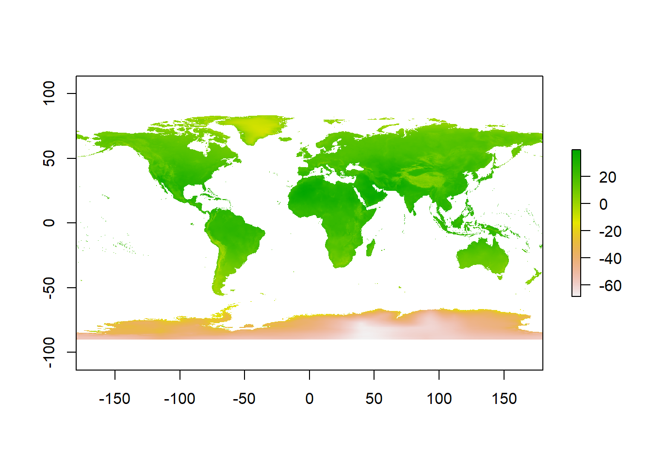
12.2.3.1 Land surface temperature
jan.temperature = stars::read_stars("data/raster/wc2.1_10m_tavg/wc2.1_10m_tavg_01.tif")

ggplot() +
  stars::geom_stars(data = jan.temperature)+
  coord_cartesian(expand = FALSE)+
  scale_fill_gradientn(colours = oce::oce.colors9A(120), na.value = "white")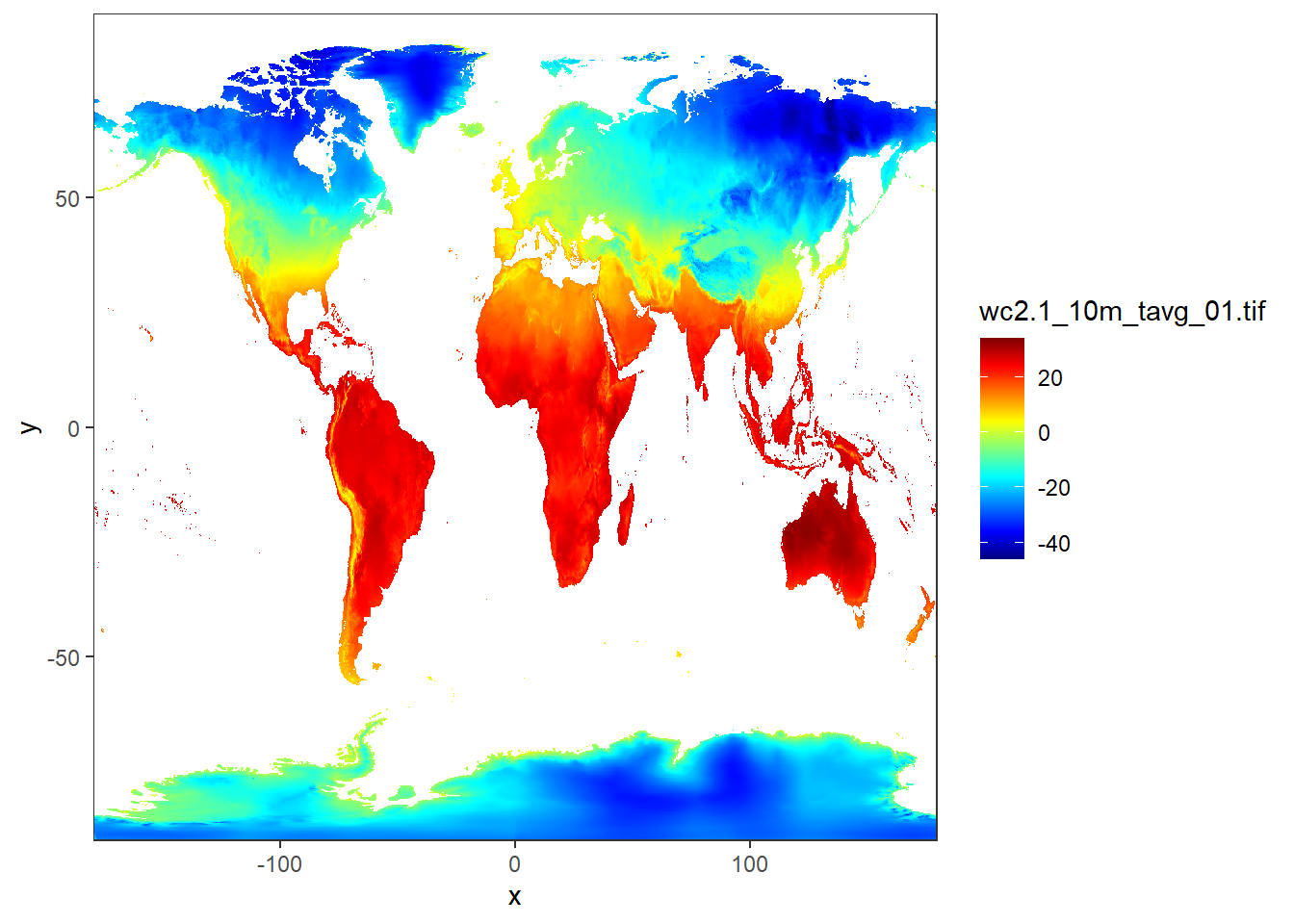
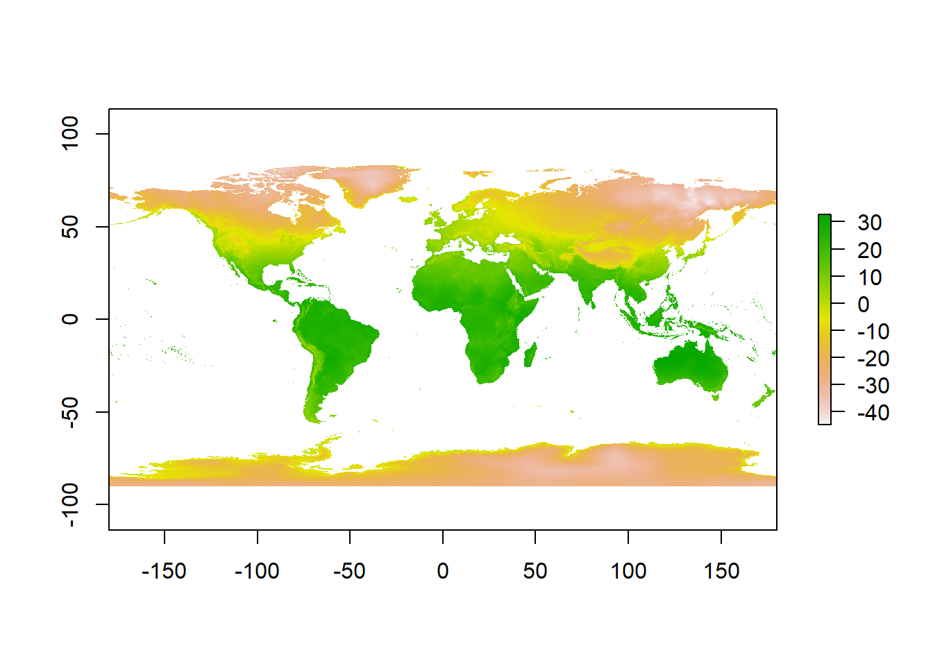
12.2.3.2 Land surface wind
jan.wind = stars::read_stars("data/raster/wc2.1_10m_wind/wc2.1_10m_wind_01.tif")

ggplot() +
  stars::geom_stars(data = jan.wind)+
  coord_cartesian(expand = FALSE)+
  scale_fill_gradientn(colours = oce::oce.colors9A(120), na.value = "white")
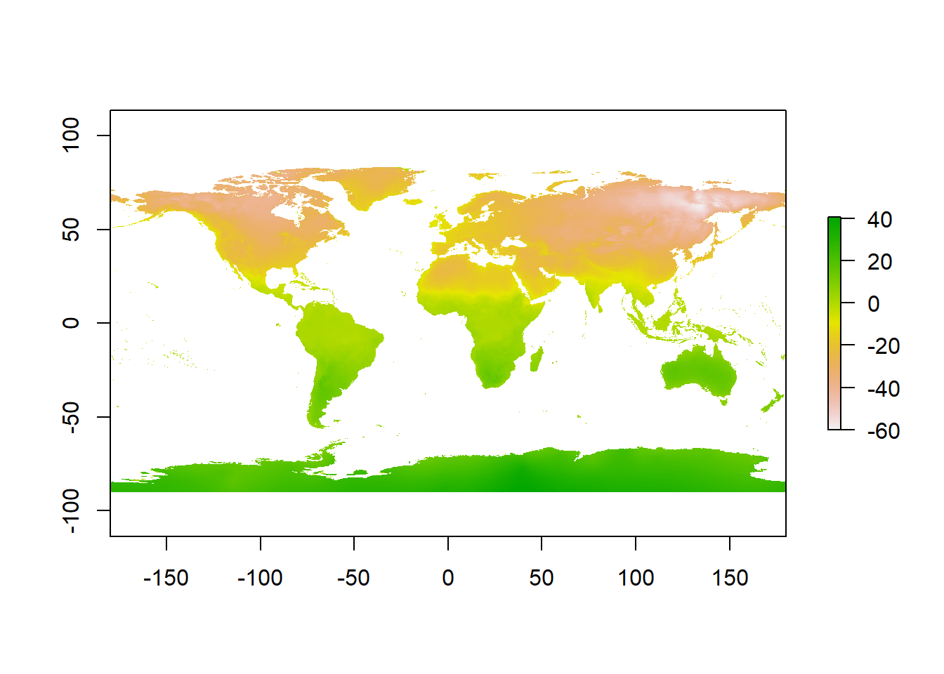
12.2.3.3 Land surface precipitation
jan.rain = stars::read_stars("data/raster/wc2.1_10m_prec/wc2.1_10m_prec_01.tif")

ggplot() +
  stars::geom_stars(data = jan.rain)+
  coord_cartesian(expand = FALSE)+
  scale_fill_gradientn(colours = oce::oce.colors9A(120), na.value = "white")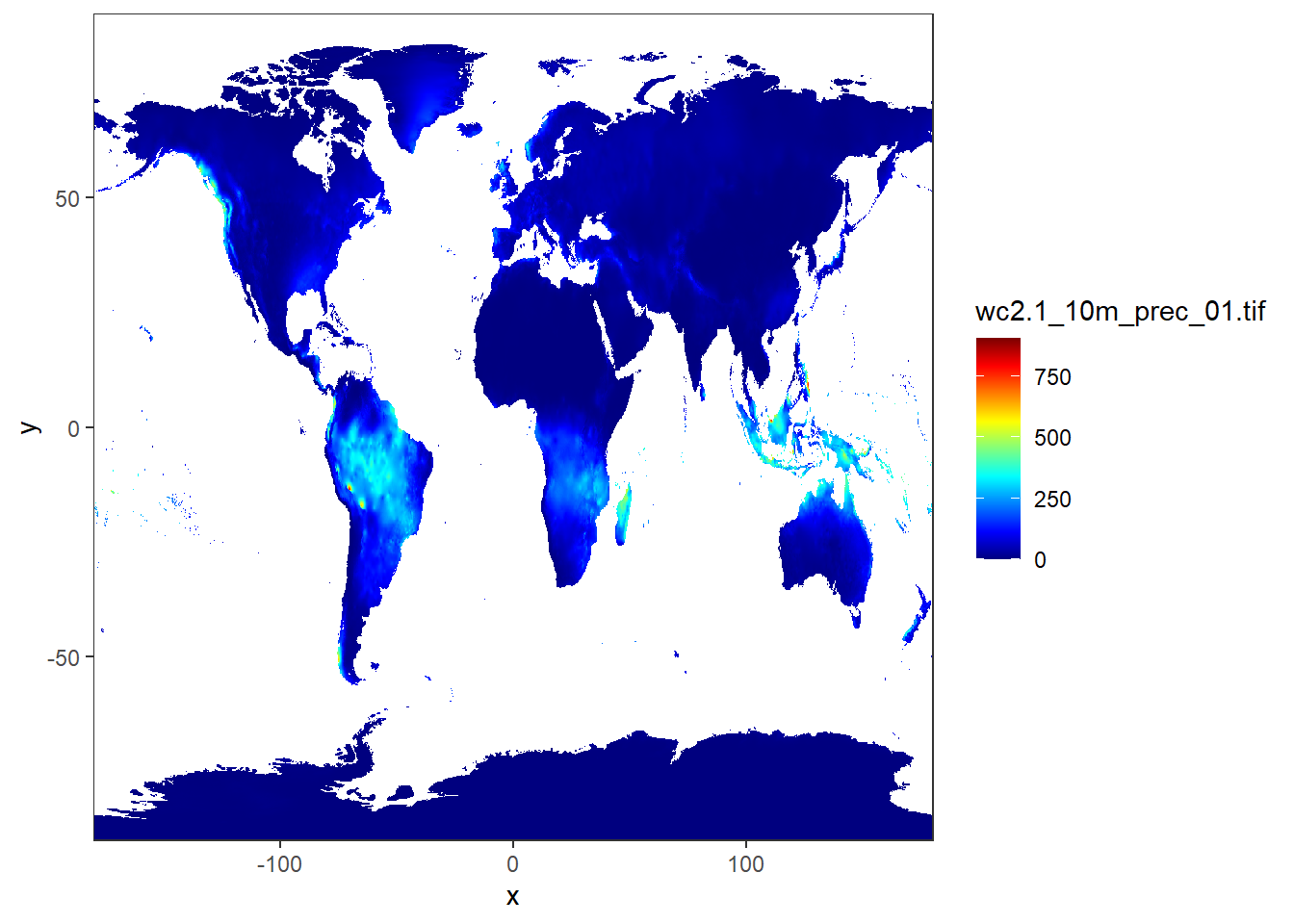

12.3 Summary
In this chapter, we learned how to load, manipulate, and analyze raster data. The things we have learned here will work as the cornerstone for doing complicated raster analysis tasks, such as applying machine learning algorithms, as we’ll be discussing in later chapters. We learned how to read and load raster data using the raster() function from the raster package in R. For multispectral images, such as Landsat images, we have learned how
12.4 Questions
Now that you’ve completed this chapter, you should be ready to answer the following questions:
- How do you load raster data in R?
- How do you change projections of rasters in R?
- How do you visualize raster in R?
- How do you reclassify rasters in R ?
- How do you clip rasters by vector data?
- How do you sample raster data using points?
References
Bauer, Robert K. 2020. Oceanmap: A Plotting Toolbox for 2D Oceanographic Data. https://CRAN.R-project.org/package=oceanmap.
Hijmans, Robert J. 2020. Raster: Geographic Data Analysis and Modeling. https://CRAN.R-project.org/package=raster.
Pierce, David. 2019. Ncdf4: Interface to Unidata netCDF (Version 4 or Earlier) Format Data Files. https://CRAN.R-project.org/package=ncdf4.