Chapter 10 Creating Geospatial Data
In previous tutorial, we learned how to use R for basic geospatial tasks, such as loading vector data, visualizing it, and stylizing it. We’ve learned the basics of GIS and vector data, how R store them, and more. This tutorial will introduce you to the creation of data and the editing functionalities of spatial data found in R. We’ll be introduced to different data sources and how to download data from one of these sites. Often, we need to create a digitized map from a printed map, and we’ll be covering that in this chapter. After this, we’ll learn how to create point, line, and polygon data using QGIS. We’ll then learn how to add features to a shapefile and how to create and use a spatial database. These skills will enable us to work more eŃciently with spatial data.
The following topics will be covered in this chapter:
- Getting data from the web
- Creating vector data
- Digitizing a map
- Working with databases
10.1 Getting data from the web
Working with geospatial data will often require us to use a spatial file that delineates country borders, roads, railways, rivers, coastlines, and so on. Sometimes, it’s hard to manage all of this data by yourself. Luckily, we can download free shapefile or vector data and raster from a number of websites for free.
One source of free vector and raster data for use in GIS is Natural Earth. Natural Earth is a public domain map dataset available at large (1:10m), medium (1:50m), and small(1:110m) scales. The Łrst two types of data contain shapefile for cultural, physical, and raster data, whereas small-scale data is available for cultural and physical data only. Figure 10.1 is a screenshot of Natural earth webpage:
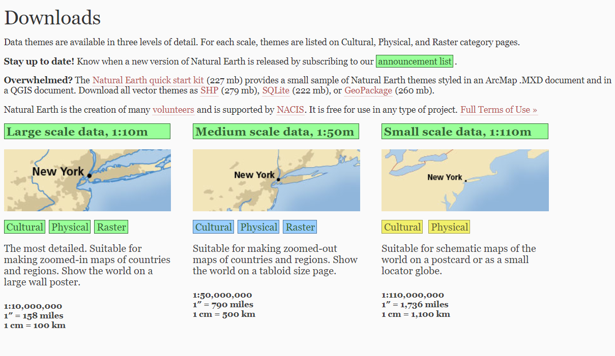
Figure 10.1: A naturalearth website preview
Rather than manual download of the dataset, We can use rnaturalearth package (South 2017), which allows us to access the Natural Earth page and dowload the data programatically. This package facilitates mapping by making natural earth map data from more easily available to R users in either sp or sf format. To use the package we need to install in our machine;
Install from CRAN :
or install the development version from GitHub using devtools.
Data to support much of the package functionality are stored in two data packages that you will be prompted to install when required if you do not do so here.
devtools::install_github("ropensci/rnaturalearthdata")
install.packages("rnaturalearthhires",
                 repos = "http://packages.ropensci.org",
                 type = "source")
10.1.1 Usage
10.1.1.1 Large Scale
Large scale data is not found in the package and you may need to download separate.
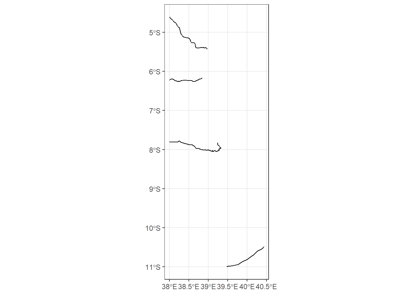
10.1.1.2 Medium Scale
coastline = rnaturalearth::ne_coastline(returnclass = "sf", scale = "medium")
countries = rnaturalearth::ne_countries(returnclass = "sf", scale = "medium")ggplot()+
geom_sf(data = countries) +
geom_sf(data = coastline)+
coord_sf(xlim = c(38.5,40.5), ylim = c(-7.,-4.5), expand = FALSE)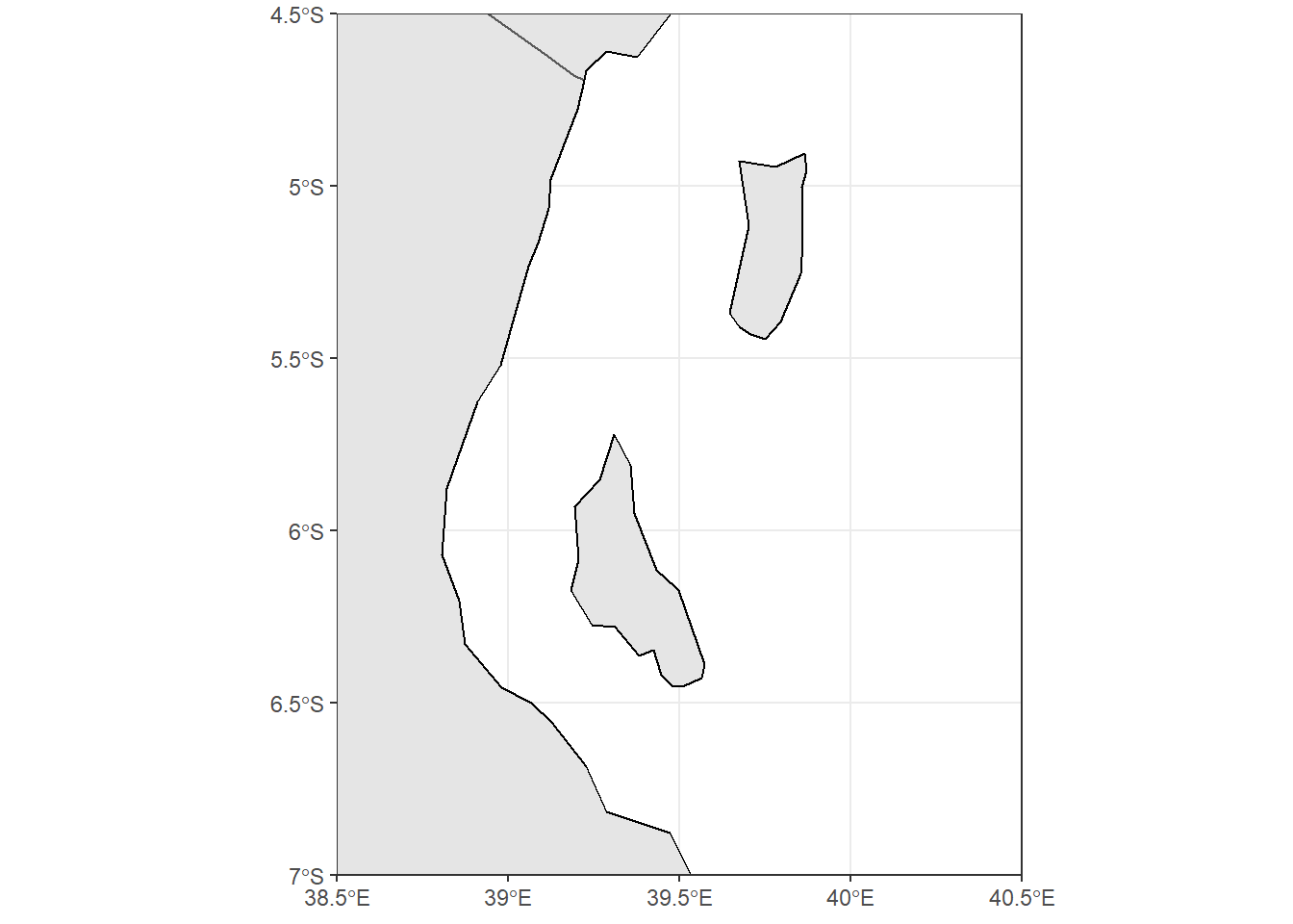
10.1.1.3 Small Scale
coastline = rnaturalearth::ne_coastline(returnclass = "sf", scale = "small")
countries = rnaturalearth::ne_countries(returnclass = "sf", scale = "small")ggplot()+
geom_sf(data = countries) +
geom_sf(data = coastline)+
coord_sf(xlim = c(38.5,40.5), ylim = c(-7.,-4.5), expand = FALSE)
10.1.2 To download Natural Earth data not already in the package
There are a wealth of other data available at the Natural Earth website. rnaturalearth has functions to help with download of these data. The function to perform that task is rnaturalearth::ne_download, which allows to specify scale, type and category and will construct the url and download the corresponding file.
10.1.2.1 Land
# rivers
land <- rnaturalearth::ne_download(scale = 10,
                                     type = 'land',
                                     category = 'physical')

sp::plot(land, col = 'blue')
10.1.2.2 Lakes
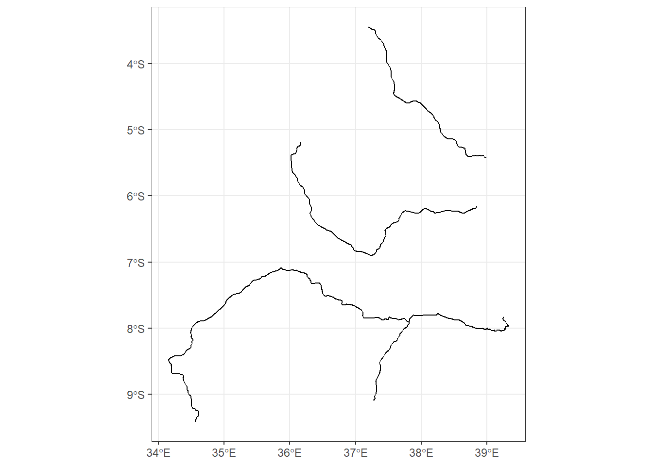
# lakes
lakes <- rnaturalearth::ne_download(scale = 10, type = 'lakes', category = 'physical')

## convert to simple feature
lakes.sf = lakes %>% st_as_sf()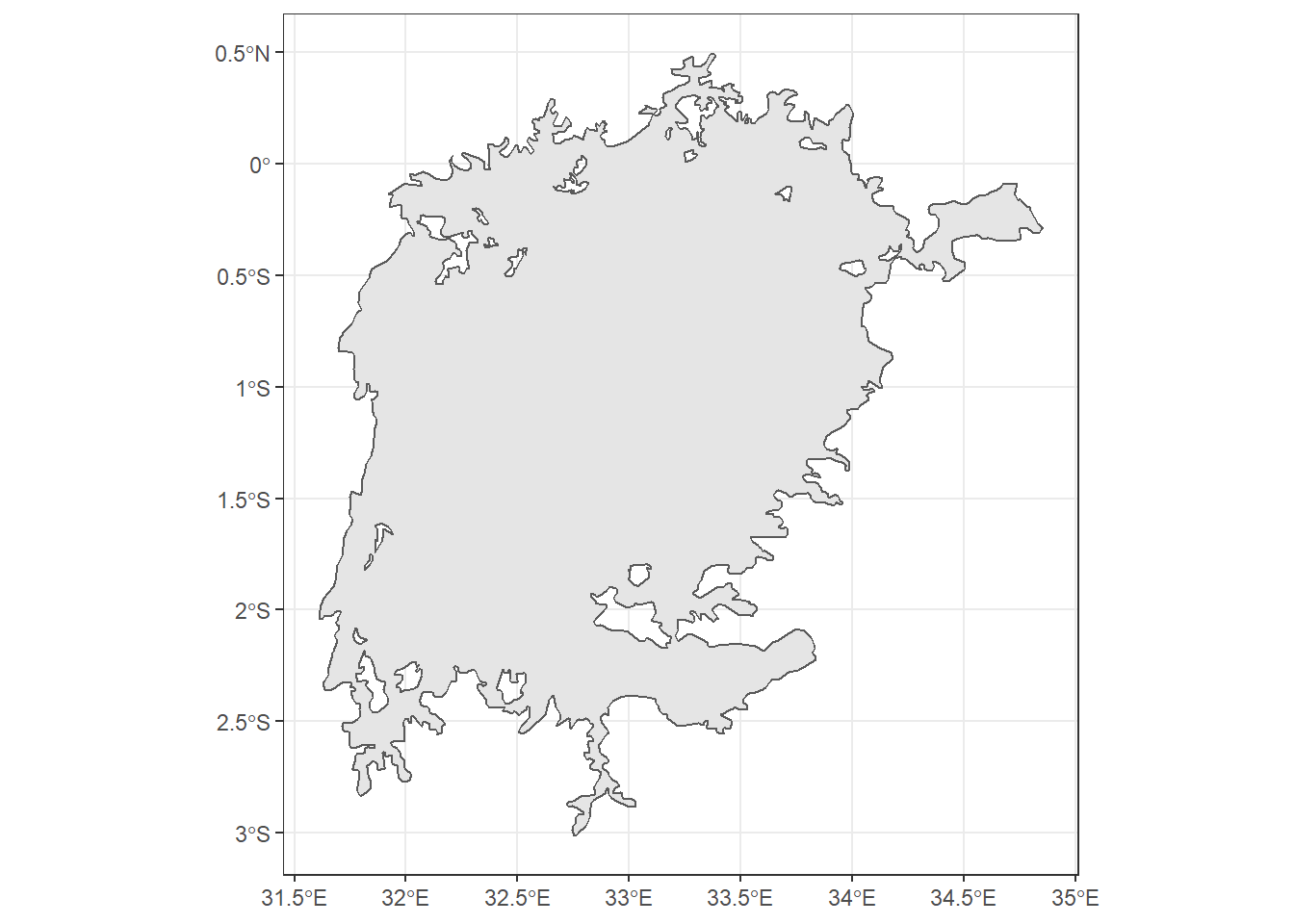
Figure 10.2: Lake Victoria
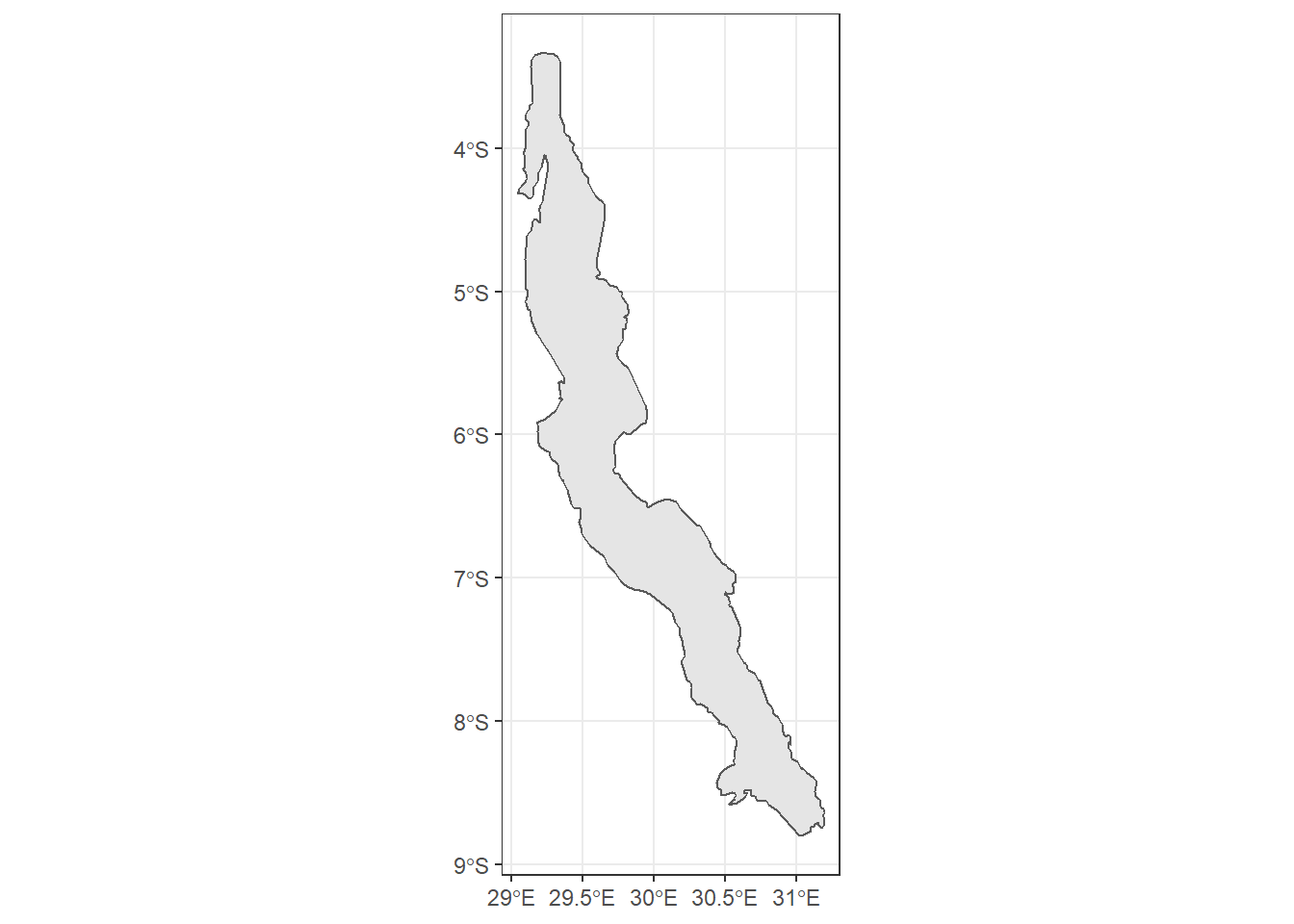
Figure 10.3: Lake Tanganyika
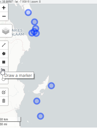
10.2 Creating Point Data
Creating point vector data is very easy in R. With the combination of leaflet (Cheng, Karambelkar, and Xie 2019) and mapedit (Appelhans, Russell, and Busetto 2020) package, you can easily create all three vectors—point, lines and polygons interactively in R. You need to have a simple feature in your working directory that the tools will borrow its geographical coordinate system. Let us start by importing the shapefile in our data folder
Once we have the points, we can use that as reference from which all layers we just wat to create will base on for its GCS
10.2.1 Creating point features
10.2.2 Creating line features
Creating line and polygon features in R is a very similar process to the workłows we followed for creating point feature. Here, we’ll look at some of the steps that we need to take in creating line feature:

10.2.3 Creating Polygon features

10.2.4 Adding features to vector data
We’ve created data of the polygon type, and we need to add features now by creating polygons and then Łlling feature attributes accordingly
10.2.5 Digitizing a map
In this section, we’ll learn how to digitize a map, which will allow us to work with this map for further spatial analysis. In doing so, we need to know the coordinates of some of the point locations on this image. We’ll use these location coordinates to digitally get coordinates of all points on the image. These points are called Ground Control Points (GCPs)
10.3 Summary
In this tutorial, we’ve learned how to create vector feature. In doing so, this tutorial showed how we can create point, line, and polygon data. Furthermore, it also covered how we can populate different features with attribute values and how we can use the Georeferencer plugin to digitize an image. We ended the tutorial by learning how create new feature from scanned digital maps.
We’ve covered just enough to proceed to the next tutorials, where we will delve deep into diferent spatial operations, spatial analysis, and more. We haven’t talked in detail about spatial databases and many other operations that could be performed using spatial databases. But the topics covered so far should have equipped you with sufficient resources to dig deeper and, in later chapters, to start applying machine learning models in spatial research cases.
10.4 Questions
- How do you create point, line and polygon features in R
- How do you digitize an image?
10.5 Further reading
We’ve shown how to create vector data but haven’t touched upon the topic of topological error correction. Furthermore, we haven’t gone into detail about the various options oŀered by the GDAL Georeferencer plugin. The book Mastering QGIS, by Menke et al, goes into detail explaining these.
References
Appelhans, Tim, Kenton Russell, and Lorenzo Busetto. 2020. Mapedit: Interactive Editing of Spatial Data in R. https://CRAN.R-project.org/package=mapedit.
Cheng, Joe, Bhaskar Karambelkar, and Yihui Xie. 2019. Leaflet: Create Interactive Web Maps with the Javascript ’Leaflet’ Library. https://CRAN.R-project.org/package=leaflet.
South, Andy. 2017. Rnaturalearth: World Map Data from Natural Earth. https://CRAN.R-project.org/package=rnaturalearth.