Chapter 2 A glimpse of R, Rstudio and Packages
This chapter is designed to help you to get started using R and RStudio, assuming no prior use of either. If you already have experience using R and RStudio, you may find some of the contents of this chapter to be a refresher - or as a chance to learn a few new things about setting up and using them. If you are looking to get started with the very basics of data loading and manipulation using the {tidyverse} (Wickham, Averick, et al. (2019)) right now, consider reading this chapter quickly and then starting with the importing data in chapter 4, reshaping data in Chapter 5 and manipulate data in chapter 6
What is R? Before we begin it is important to consider what R is. R is a programming language for statistical computing and graphics (R Core Team 2020). R is a programming language which is highly used in data science. R is becoming more and more popular due to two major reasons:
- R is open source.
- R has most of the latest statistical methods.
R has a base language that allows a user to program almost anything they like. Of course to do this takes a lot of time and trial-and-error. This can be easily solved when you consider that there are also many user defined packages and functions.
In fact there are over 15,000 packages as of January 2021 and this number is growing exponentially.
Should you use R? You may want to ask yourself these questions?
- Do I need a tool to work with data?
- Am I looking for something cost effective?
- Do I want to learn to code in a language that gives me a great deal of freedom?
- Would I like to be able to easily define my own procedures and functions?
- If you answered Yes to any of those question than it may be worthwhile for you to start using R.
We will begin to layout a bit more framework on why so many data scientists choose to work with R over every other language.
2.1 The Data Analysis Workflow
We begin by looking at the Data Analysis workflow presented in figure 2.1, a concept by Hadley Wickham. The diagram shows the natural flow of how we work with data and perform research. We will begin to explore what this means as we continue.
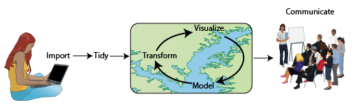
Figure 2.1: A conceptual diagram of data science model
2.1.1 Data Wrangling
The first steps we take in any Data Analysis is Data Wrangling. Before we can do any kind of analysis we need to be able to collect our data. Sometimes this comes in from one source but many times this comes from multiple data sources. Once we have this data we find that very rarely is it ever in a useful form. In fact Wickham and Grolemund (2016) suggest that this data preparation of cleaning may take up to 80% of the time.
2.1.2 Importing Data
When it comes to importing your data R is very powerful. R can grab data from many courses including
- .csv, .txt. .xls, ….
- SPSS, SAS, Stata
- Web Scraping
- Databases
2.1.3 Tidying Data
Tidying Data is the process in making data useful. In this concept we have ecah column of data represent a variable and each row of data represents a single observation. This format is quite useful for data analysis. In this course we will rely heavily on the tidyr package (Wickham 2020).
2.1.4 Transforming Data
Once we have data into R and begin to tidy the data we usually need to transform multiple aspects of the data. R has many tools that allow a user to manipulate and transform data. R is one of the most capable languages to explore and analyze data. With over 15,000 packages it can be hard to find models or plots that do not already have multiple functions in R.
2.1.5 Visualizing Data
There are multiple ways to vizualize data in R. The base graphics are easy to use and outperform Stata, SAS and SPSS. In this course we will focus on using the ggplot2 package (Wickham 2016). This package is actually a language for graphics and once a user becomes familiar and proficient you can create professional and publication quality graphs.
2.1.6 Models
Once you have made your questions sufficiently precise, you can use a model to answer them. Models are a fundamentally mathematical or computational tool, so they generally scale well. Even when they don’t, it’s usually cheaper to buy more computers than it is to buy more brains! But every model makes assumptions, and by its very nature a model cannot question its own assumptions. That means a model cannot fundamentally surprise you.
2.1.7 Data Collaboration and Publishing
In every field it is key to be able to communicate what we learn and publish this work so that it can be beneficial to others. This is an absolutely critical part of any data analysis project. It doesn’t matter how well your models and visualisation have led you to understand the data unless you can also communicate your results to others.
Surrounding all these tools is programming, this is where R language has great power.
2.2 Installation
2.2.1 Installing R
To download R, go to CRAN, the comprehensive R archive network. CRAN is composed of a set of mirror servers distributed around the world and is used to distribute R and R packages. Don’t try and pick a mirror that’s close to you: instead use the cloud mirror, https://cloud.r-project.org, which automatically figures it out for you.
A new major version of R comes out once a year, and there are 2-3 minor releases each year. It’s a good idea to update regularly. Upgrading can be a bit of a hassle, especially for major versions, which require you to reinstall all your packages, but putting it off only makes it worse.
- Go to https://cran.r-project.org/
- Click Download R for Mac/Windows.
- Click the link appropriate for your system (Linux, Mac, Windows)
Don’t worry; you will not mess anything up if you download (or even install!) the wrong file. Once you’ve installed R, you can get started.
2.2.2 Installing RStudio
RStudio is an integrated development environment, or IDE, for R programming (RStudio Team 2015). RStudio is a set of integrated tools that allows for a more user-friendly experience for using R. Although you will likely use RStudio as your main console and editor, you must first install R, as RStudio uses R behind the scenes. Both R and RStudio are freely-available, cross-platform, and open-source.
Download and install it from http://www.rstudio.com/download. RStudio is updated a couple of times a year. When a new version is available, RStudio will let you know. It’s a good idea to upgrade regularly so you can take advantage of the latest and greatest features.
- Go to https://www.rstudio.com/products/rstudio/download/
- Click Download under RStudio Desktop.
- Click the link appropriate for your system (Linux, Mac, Windows)
- Follow the instructions of the Installer.
2.2.3 Rstudio Layout
Whenever we want to work with R, we’ll open RStudio. RStudio interfaces directly with R, and is an Integrated Development Environment (IDE). This means that RStudio comes with built-in features that make using R a little easier. When you start RStudio, you’ll see four key panels in the interface shown in figure ??. We’ll refer to these four “panes” as the editor, the Console, the Environment, and the Files panes. The large square on the left is the Console pane, the square in the top right is the Environment pane, and the square in the bottom right is the Files pane. As you work with R more, you’ll find yourself using the tabs within each of the panes.
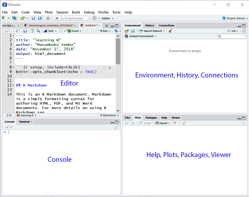
Figure 2.2: The interface of Rstudio IDE with four key panels
When we create a new file, such as an R script, an R Markdown file, or a Shiny app, RStudio will open a fourth pane, known as the source or editor pane. The source pane should show up as a square in the top left. We can open up an .R script in the source pane by going to File, selecting New File, and then selecting R Script:
2.2.4 Installing Packages
This section will briefly go over installing packages that’s used throughout this book. An R package is a collection of functions, data, and documentation that extends the capabilities of base R. Using packages is key to the successful use of R. The majority of the packages that you will learn in this course are part of the so-called tidyverse. The packages in the tidyverse share a common philosophy of data and R programming, and are designed to work together naturally.
The Tidyverse (Wickham, Averick, et al. 2019) packages form a core set of functions that will allow us to perform most any type of data cleaning or analysis we will need to do. We will use the following packages from the tidyverse
- ggplot2—for data visualisation.
- dplyr—for data manipulation.
- tidyr—for data tidying.
- readr—for data import.
- purrr—for functional programming.
- tibble—for tibbles, a modern re-imagining of data frames.
For us to use tidyverse and any other package that is not included in Base R, we must install them first. The easiest way to install packages is to use the install.packages() command. For example, let’s go ahead and install the tidyverse package on your machine:
On your own computer, type that line of code in the console, and then press enter to run it. R will download the packages from CRAN and install them on to your computer. If you have problems installing, make sure that you are connected to the internet, and that https://cloud.r-project.org/ isn’t blocked by your firewall or proxy.
2.2.5 Other packages
There are many other excellent packages that are not part of the tidyverse, because they solve problems in a different domain, or are designed with a different set of underlying principles. This doesn’t make them better or worse, just different. In other words, the complement to the tidyverse is not the messyverse, but many other universes of interrelated packages (Wickham and Grolemund 2016). As you tackle more data science projects with R, you’ll learn new packages and new ways of thinking about data. In this course we’ll use several data packages from outside the tidyverse:
2.2.6 Loading installed packages
With exception to base R package, add on package that are installed must be called with either library or require functions to make their tools accessible in R session. Let’s us load the tidyverse package we just installed
You notice that when we load tidyverse, it popup a notification message showing the loaded packages and the conflicts they bring in. These conflicts happen when packages have functions with the same names as other functions. This is OK when you prefer the function in a package like tidyverse rather than some other function. Basically the last package loaded in will mask over other functions if they have common names.
2.2.7 Exploring R with the {swirl} Package
If you were able to install the {dataedu} package without any issues or concerns, and you’re eager to get started exploring everything that R can do, you can supplement your learning through {swirl} (https://swirlstats.com/students.html).
You can install {swirl} by running the following code:
{swirl} is set of packages (see more on packages in Chapter 6) that you can download, providing an interactive method for learning R by using R in the RStudio Console.
Since you’ve already installed R, RStudio, and the {swirl} package, you can follow the instructions on the {swirl} webpage or run the following code in your console pane to get started with a beginner-level course in {swirl}:
There are multiple courses available on {swirl}, and you can access them by installing them and then running the swirl() command in your console.
We are not affiliated with {swirl} in any way, nor is it required to use {swirl} in order to progress through this text, but it’s a great resource that we want to make sure is on your radar!
2.2.8 Conclusion
It would be impossible for us to cover everything you can do with R in a single chapter of a book, but it is our hope that this chapter gives you a strong foundation from which to explore both subsequent chapters as well as additional R resources. Appendix extends some of the techniques introduced in
References
R Core Team. 2020. R: A Language and Environment for Statistical Computing. Vienna, Austria: R Foundation for Statistical Computing. https://www.R-project.org/.
RStudio Team. 2015. RStudio: Integrated Development Environment for R. Boston, MA: RStudio, Inc. http://www.rstudio.com/.
Wickham, Hadley. 2016. Ggplot2: Elegant Graphics for Data Analysis. Springer-Verlag New York. https://ggplot2.tidyverse.org.
Wickham, Hadley. 2020. Tidyr: Tidy Messy Data. https://CRAN.R-project.org/package=tidyr.
Wickham, Hadley, Mara Averick, Jennifer Bryan, Winston Chang, Lucy D’Agostino McGowan, Romain François, Garrett Grolemund, et al. 2019. “Welcome to the tidyverse.” Journal of Open Source Software 4 (43): 1686. https://doi.org/10.21105/joss.01686.
Wickham, Hadley, and Garrett Grolemund. 2016. R for Data Science: Import, Tidy, Transform, Visualize, and Model Data. " O’Reilly Media, Inc.".