Chapter 5 Reshaping data with tidyr
5.1 What is Tidy Data?
Most statistical datasets are data frames made up of rows and columns. The columns are almost always labeled and the rows are sometimes labeled. One of the key task in data preparation is to organize a dataset in a way that makes analysis and plottng easier. In practice, the data is often not stored like that and the data comes to us with repeated observations included on a single row. This is often done as a memory saving technique or because there is some structure in the data that makes the ‘wide’ format attractive. As a result, we need a way to convert data from wide1 to long2 and vice-versa (Semba and Peter 2020).
Structuring data frames to have the desired shape can be the most daunting part of statistical analysis, visualization, and modeling. Several studies reported that 80% of data analysis is spent on the cleaning and preparing data. Tidy in this context means organize the data in a presentable and consistent format that facilitate data analysis and visualization. When you are doing data preparation in R for analysis or plottng, the first thing you do is a thoroughly mental thought on the desired structure of that data frame. You need to determine what each row and column will represent, so that you can consistently and clearly manipulate that data (e.g., you know what you will be selecting and what you will be filtering).
There are basically three principles that we can follow to make a tidy dataset.
- First each variable must have its own a column,
- second each observation must have its own row, and
- finally, each cell must have its own value.
The tidyr package is designed to structure and work with data frames that follow three principles of tidy data. There are advantages of using tidy data in R.
- First, having a consistent, uniform data structure is very important. Popular packages like dplyr (Wickham, François, et al. 2020), ggplot2 (Wickham 2016), and all the other packages in the tidyverse (Wickham, Averick, et al. 2019) and their extensions like sf (Pebesma 2018), metR (Campitelli 2019), ggspatial (Dunnington 2020), ggrepel (Slowikowski 2020) etc are designed to work with tidy data (Wickham 2020). So consistent of tidy data ensure efficient processing, analysis and plotting of data.
- Third, placing variables into columns, facilities easy vectorization in R.
Unfortunate, Many datasets that you receive are untidy and will require some work on your end. There are several reasons why a dataset is messy.
- Often times the people who created the dataset aren’t familiar with the principles of tidy data.
- Another common reason that most datasets are messy is that data is often organized to facilitate something other than analysis.
- Data entry is perhaps the most common of the reasons that fall into this category.
To make data entry as easy as possible, people will often arrange data in ways that aren’t tidy. So, many datasets require some sort of tidying before you can begin your analysis.
As Wickham and Grolemund (2016) put it tidy data means that yo can plot or summarize the data efficiently. In othet words, it comes down to which data is represented as columns in a data frame and which is not.In principle, this means that there is column in the data frame that you can work with for the analysis you want to do. For example, if I want to look at the ctd dataset and see how the fluorescence varies among station in the upper water surface, we simply plot a boxplot of the station column against the fluorescence column shown in figure 5.1
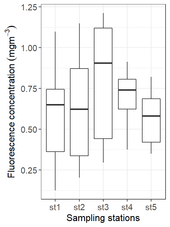
Figure 5.1: Fluorescence variation against stations
This works because I have a column for the x-axis and another for the y-axis. But what happens if I want to plot the different measurements of the irises to see how those are? Each measurement is a separate column. They are Petal.Length, Petal.Width, and so on.Now I have a bit of a problem because the different measurements are in different columns in my data frame. I cannot easily map them to an x-axis and a y-axis.The tidyr package addresses that. It contains functions for both mapping columns to values—, widely recognised as long format and for mapping back from values to columns—wide format.
We are going to look for the function that are regularly used to tidy the data frames. These inlude:
- Gathering
- Spreading
- Separating
- Uniting
5.2 Gather—from wide to long format.
Look at example of dataset. It has one common problem that the column names are not variables but rather values of a variable. In the table 5.1, the columns are actually values of the variable pressure. Each row in the existing table actually represents five observations from each station.
| station | 10 | 20 | 30 | 40 | 50 | 60 | 70 | 80 | 90 | 100 | 110 |
|---|---|---|---|---|---|---|---|---|---|---|---|
| st1 | 0.599 | 0.678 | 0.729 | 0.693 | 0.752 | 1.098 | 0.857 | 0.481 | 0.313 | 0.221 | 0.138 |
| st2 | 0.631 | 0.733 | 0.992 | 1.114 | 0.988 | 0.715 | 0.496 | 0.524 | 0.280 | 0.277 | 0.225 |
| st3 | 0.980 | 0.934 | 1.149 | 1.200 | 1.187 | 1.035 | 0.854 | 0.530 | 0.437 | 0.347 | 0.324 |
| st4 | NA | 0.623 | 0.603 | 0.742 | 0.724 | 0.799 | 0.914 | 0.819 | 0.801 | 0.692 | 0.444 |
| st5 | NA | 0.350 | 0.415 | 0.421 | 0.566 | 0.592 | 0.591 | 0.634 | 0.751 | 0.774 | 0.575 |
The tidyr package can be used to gather these existing columns into a new variable. In this case, we need to create a new column called pressure and then gather the existing values in the these variable columns into the new pressure variable
# A tibble: 55 x 3
   station depth `fluorescence `
   <chr>   <chr>           <dbl>
 1 st1     10              0.599
 2 st2     10              0.631
 3 st3     10              0.98
 4 st4     10             NA
 5 st5     10             NA
 6 st1     20              0.678
 7 st2     20              0.733
 8 st3     20              0.934
 9 st4     20              0.623
10 st5     20              0.350
# ... with 45 more rows
As you can see from the chunk above, there are three arguments required in the gather() function. First is the key, which takes the variable names. Second, the value—the name of the variable whose values are spread over the cells. Finnaly, then you specify the set of columns that hold the values and not the variable names
5.3 spread—from long to wide format
A second tidy tool is spread(), which does the opposite of gather() function. It is used to convert a long format data frame to wide format. What this function does is to spread observation across multiple rows.
# A tibble: 5 x 12
  station   `10` `100` `110`  `20`  `30`  `40`  `50`
  <chr>    <dbl> <dbl> <dbl> <dbl> <dbl> <dbl> <dbl>
1 st1      0.599 0.221 0.138 0.678 0.729 0.693 0.752
2 st2      0.631 0.277 0.225 0.733 0.992 1.11  0.988
3 st3      0.98  0.347 0.324 0.934 1.15  1.20  1.19
4 st4     NA     0.692 0.444 0.623 0.603 0.742 0.724
5 st5     NA     0.774 0.575 0.350 0.415 0.421 0.566
# ... with 4 more variables: `60` <dbl>, `70` <dbl>,
#   `80` <dbl>, `90` <dbl>
The spread() function takes two arguments: the column that contains variable names, known as the key and
a column that contains values from multiple variables – the value.
5.4 separate columns
Another common in tidyr package is a separate ()function, which split the variable into two or more variables. For example, the dataset below has a date column that actually contains the date and time variables separated by a space.
# A tibble: 115 x 12
   station time                  lon   lat pressure
   <chr>   <dttm>              <dbl> <dbl>    <dbl>
 1 st1     2004-08-18 15:27:46  40.6 -10.5        5
 2 st1     2004-08-18 15:27:46  40.6 -10.5       10
 3 st1     2004-08-18 15:27:46  40.6 -10.5       15
 4 st1     2004-08-18 15:27:46  40.6 -10.5       20
 5 st1     2004-08-18 15:27:46  40.6 -10.5       25
 6 st1     2004-08-18 15:27:46  40.6 -10.5       30
 7 st1     2004-08-18 15:27:46  40.6 -10.5       35
 8 st1     2004-08-18 15:27:46  40.6 -10.5       40
 9 st1     2004-08-18 15:27:46  40.6 -10.5       45
10 st1     2004-08-18 15:27:46  40.6 -10.5       50
# ... with 105 more rows, and 7 more variables:
#   temperature <dbl>, salinity <dbl>, oxygen <dbl>,
#   fluorescence <dbl>, spar <dbl>, par <dbl>,
#   density <dbl>
We use the separate() function splits the datetime column into two variables: date and time
# A tibble: 115 x 13
   station Date  Time    lon   lat pressure
   <chr>   <chr> <chr> <dbl> <dbl>    <dbl>
 1 st1     2004~ 15:2~  40.6 -10.5        5
 2 st1     2004~ 15:2~  40.6 -10.5       10
 3 st1     2004~ 15:2~  40.6 -10.5       15
 4 st1     2004~ 15:2~  40.6 -10.5       20
 5 st1     2004~ 15:2~  40.6 -10.5       25
 6 st1     2004~ 15:2~  40.6 -10.5       30
 7 st1     2004~ 15:2~  40.6 -10.5       35
 8 st1     2004~ 15:2~  40.6 -10.5       40
 9 st1     2004~ 15:2~  40.6 -10.5       45
10 st1     2004~ 15:2~  40.6 -10.5       50
# ... with 105 more rows, and 7 more variables:
#   temperature <dbl>, salinity <dbl>, oxygen <dbl>,
#   fluorescence <dbl>, spar <dbl>, par <dbl>,
#   density <dbl>
The separate() function accepts arguments for the name of the variable to separate. You also need to specify the names of the variable to separate into, and an optional separator.
5.5 unite columns
The unite()function is the exact opposite of separate() in that it combines multiple columns into a single column. While not used nearly as often as separate() , there may be times when you need the functionality provided by unite(). For example, we can combine the variable Date and Time to form siku.muda, and separate them with :-: symbol between the two variables.
# A tibble: 115 x 12
   station siku_muda   lon   lat pressure temperature
   <chr>   <chr>     <dbl> <dbl>    <dbl>       <dbl>
 1 st1     2004-08-~  40.6 -10.5        5        25.2
 2 st1     2004-08-~  40.6 -10.5       10        25.1
 3 st1     2004-08-~  40.6 -10.5       15        25.1
 4 st1     2004-08-~  40.6 -10.5       20        25.0
 5 st1     2004-08-~  40.6 -10.5       25        24.9
 6 st1     2004-08-~  40.6 -10.5       30        24.9
 7 st1     2004-08-~  40.6 -10.5       35        24.9
 8 st1     2004-08-~  40.6 -10.5       40        24.9
 9 st1     2004-08-~  40.6 -10.5       45        24.8
10 st1     2004-08-~  40.6 -10.5       50        24.6
# ... with 105 more rows, and 6 more variables:
#   salinity <dbl>, oxygen <dbl>, fluorescence <dbl>,
#   spar <dbl>, par <dbl>, density <dbl>
References
Campitelli, Elio. 2019. MetR: Tools for Easier Analysis of Meteorological Fields. https://CRAN.R-project.org/package=metR.
Dunnington, Dewey. 2020. Ggspatial: Spatial Data Framework for Ggplot2. https://CRAN.R-project.org/package=ggspatial.
Pebesma, Edzer. 2018. “Simple Features for R: Standardized Support for Spatial Vector Data.” The R Journal 10 (1): 439–46. https://doi.org/10.32614/RJ-2018-009.
Semba, Masumbuko, and Nyamisi Peter. 2020. Wior: Easy Tidy and Process Oceanographic Data.
Slowikowski, Kamil. 2020. Ggrepel: Automatically Position Non-Overlapping Text Labels with ’Ggplot2’. https://CRAN.R-project.org/package=ggrepel.
Wickham, Hadley. 2016. Ggplot2: Elegant Graphics for Data Analysis. Springer-Verlag New York. https://ggplot2.tidyverse.org.
Wickham, Hadley. 2020. Tidyr: Tidy Messy Data. https://CRAN.R-project.org/package=tidyr.
Wickham, Hadley, Mara Averick, Jennifer Bryan, Winston Chang, Lucy D’Agostino McGowan, Romain François, Garrett Grolemund, et al. 2019. “Welcome to the tidyverse.” Journal of Open Source Software 4 (43): 1686. https://doi.org/10.21105/joss.01686.
Wickham, Hadley, Romain François, Lionel Henry, and Kirill Müller. 2020. Dplyr: A Grammar of Data Manipulation. https://CRAN.R-project.org/package=dplyr.
Wickham, Hadley, and Garrett Grolemund. 2016. R for Data Science: Import, Tidy, Transform, Visualize, and Model Data. " O’Reilly Media, Inc.".