Chapter 9 Feature Representation
In tutorial 3, we learned how R handles data and went further to create data frame, a fundamental data structure in R. In this tutorial we expand a bit on data frame and see how the geographical feature are presented in R. In Geographical Information System (GIS), every dataset is associated with a coordinate system, which is a system for representing the location of different geographical features and different measurements.
Geographic data, geospatial data or geographic information is data that identifies the location of features on Earth. According to Lovelace, Nowosad, and Muenchow (2019), these spatial entities can be represented in a GIS as a vector data model or a raster data model.
9.1 Vector
Vector data is good for representing categorical and multivariate data. It also has attribute tables where every record or row corresponds to a feature or an object and every column corresponds to different attributes. Vector data has three different geometric primitives types: points, lines, and polygons.
9.1.1 A point
A point is composed of one coordinate pair representing a specific location in a coordinate system. Points represented in figure 9.1 are the most basic geometric primitives having no length or area. By definition a point can’t be “seen” since it has no area; but this is not practical if such primitives are to be mapped. So points on a map are represented using symbols that have both area and shape (e.g. circle, square, plus signs). We seem capable of interpreting such symbols as points, but there may be instances when such interpretation may be ambiguous (e.g. is a round symbol delineating the area of a round feature on the ground such as a large oil storage tank or is it representing the point location of that tank?).
stations = tibble(lon = c(39.094923,39.186061, 39.335302),
                  lat = c(-6.283669, -6.212201,-6.279278),
                  names = c("A", "B", "C"))
stations %>%
ggplot(aes(x = lon, y = lat))+
geom_point(size = 3) +
ggrepel::geom_text_repel(aes(label = names))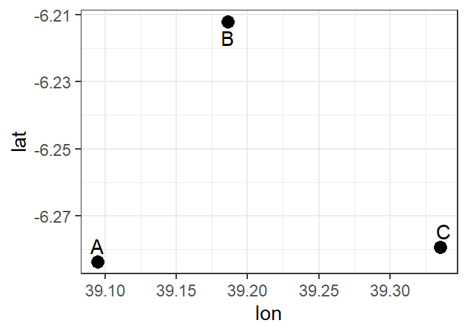
Figure 9.1: Point objects serves as sampling stations defined by their X and Y coordinate values and labelled with letters
9.1.2 Polyline
A polyline as presented in figure 9.1 is composed of a sequence of two or more coordinate pairs called vertices. A vertex is defined by coordinate pairs, just like a point, but what differentiates a vertex from a point is its explicitly defined relationship with neighboring vertices. A vertex is connected to at least one other vertex. Like a point, a true line can’t be seen since it has no area. And like a point, a line is symbolized using shapes that have a color, width and style (e.g. solid, dashed, dotted, etc…). Roads and rivers are commonly stored as polylines in a GIS.
stations %>%
  ggplot(aes(x = lon, y = lat)) +
  geom_line(color = "red", size = 1.2)+
  geom_point(size = 3)+
  ggrepel::geom_text_repel(aes(label = names))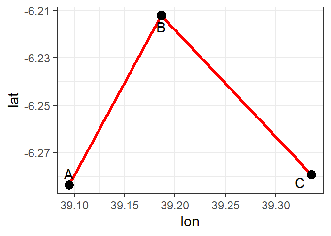
Figure 9.2: A simple polyline object defined by connected vertices
9.1.3 Polygon
A polygon is composed of three or more line segments whose starting and ending coordinate pairs are the same. Sometimes you will see the words lattice or area used in lieu of ‘polygon’. Polygons shown in figure 9.3 represent both length (i.e. the perimeter of the area) and area. They also embody the idea of an inside and an outside; in fact, the area that a polygon encloses is explicitly defined in a GIS environment. If it isn’t, then you are working with a polyline feature. If this does not seem intuitive, think of three connected lines defining a triangle: they can represent three connected road segments (thus polyline features), or they can represent the grassy strip enclosed by the connected roads (in which case an ‘inside’ is implied thus defining a polygon).
stations %>%
  ggplot(aes(x = lon, y = lat)) +
  geom_polygon(color = "red", size = 1.2, fill = "red", alpha = .12)+
  geom_point(size = 3)+
  ggrepel::geom_text_repel(aes(label = names))
Figure 9.3: A simple polygon object defined by an area enclosed by connected vertices
9.2 Raster
Raster data is used for continuous data and stores data in a grid-like arrangement. A raster data model uses an array of cells, or pixels, to represent real-world objects. Raster or “gridded” data are stored as a grid of values which are rendered on a map as pixels. Each pixel value represents an area on the Earth’s surface. Raster datasets are commonly used for representing and managing imagery, sea surface temperatures, chlorophyll-a concentration, sea surface height, wind speeed and direction, elevation and bathymetry and numerous other entities.
A raster can be thought of as a special case of an area object where the area is divided into a regular grid of cells. But a regularly spaced array of marked points may be a better analogy since rasters are stored as an array of values where each cell is defined by a single coordinate pair inside of most GIS environments.
Implicit in a raster data model is a value associated with each cell or pixel. This is in contrast to a vector model that may or may not have a value associated with the geometric primitive.
stations %>%
  ggplot(aes(x = lon, y = lat)) +
  geom_polygon(color = "red", size = 1.2, fill = "red", alpha = .12)+
  geom_point(size = 3)+
  ggrepel::geom_text_repel(aes(label = names))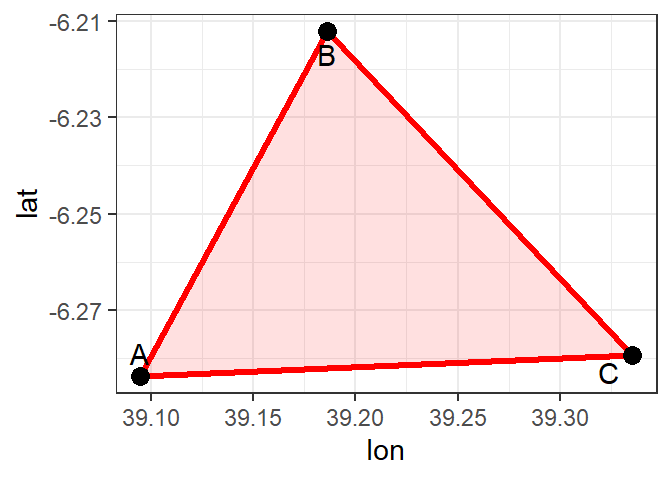
Figure 9.4: A simple polygon object defined by an area enclosed by connected vertices
9.3 Important GIS data formats
In tutorial 9 we learn some types of geographical data and how to create them. In this tutorial we are going to import already created spatial data into our session and start working on them. There are a number of commonly used geographic data formats that store vector and raster data that you will come across during this course and it’s important to understand what they are, how they represent data and how you can use them.
9.3.1 Shapefiles
Geographic data can be represented using a data storage format called shapefile that stores the location, shape, and attributes of geographic features such as points, lines and polygons. A shapefile is not a unique file, but consists of a collection of related files that have different extensions and a common name and are stored in the same directory. A shapefile has three mandatory files with extensions .shp, .shx, and .dbf:
Shapefiles were developed by ESRI, one of the first and now certainly the largest commercial GIS company in the world. Despite being developed by a commercial company, they are mostly an open format and can be used (read and written) by a host of GIS Software applications.
A shapefile is actually a collection of files –– at least three of which are needed for the shapefile to be displayed by GIS software. They are:
.shp- the file which contains the feature geometry.shx- an index file which stores the position of the feature IDs in the .shp file.dbf- the file that stores all of the attribute information associated with the coordinates – this might be the name of the shape or some other information associated with the feature.prj- the file which contains all of the coordinate system information (the location of the shape on Earth’s surface). Data can be displayed without a projection, but the .prj file allows software to display the data correctly where data with different projections might be being used
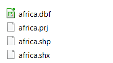
Figure 9.5: Essential files for constituting a shapefile
9.3.2 Raster
Most raster data is now provided in GeoTIFF (.tiff) format, which stands for Geostarionary Earth Orbit Tagged Image File. The GeoTIFF data format was created by NASA and is a standard public domain format. All necessary information to establish the location of the data on Earth’s surface is embedded into the image. This includes: map projection, coordinate system, ellipsoid and datum type.
9.3.3 Attribute Tables
Non-spatial information associated with a spatial feature is referred to as an attribute. A feature on a GIS map is linked to its record in the attribute table by a unique numerical identifier (ID). Every feature in a layer has an identifier. It is important to understand the one-to-one or many-to-one relationship between feature, and attribute record. Because features on the map are linked to their records in the table, many GIS software will allow you to click on a map feature and see its related attributes in the table.
Raster data can also have attributes only if pixels are represented using a small set of unique integer values. Raster datasets that contain attribute tables typically have cell values that represent or define a class, group, category, or membership. NOTE: not all GIS raster data formats can store attribute information; in fact most raster datasets you will work with in this course will not have attribute tables.
9.3.4 Geodatabase
A geodatabase is a collection of geographic data held within a database. Geodatabases were developed by ESRI to overcome some of the limitations of shapefiles. They come in two main types: Personal (up to 1 TB) and File (limited to 250 - 500 MB), with Personal Geodatabases storing everything in a Microsoft Access database (.mdb) file and File Geodatabases offering more flexibility, storing everything as a series of folders in a file system. In the example below we can see that the FCC_Geodatabase (left hand pane) holds multiple points, lines, polygons, tables and raster layers in the contents tab.
9.4 Coordinate reference systems
An important aspect of spatial data is the coordinate reference system (CRS) that is used to represent object on earth’s surface. A CRS permits us to know the origin and the unit of measurement of the coordinates. Moreover, in the case of dealing with multiple data, knowledge of CRS permits to transform all data to a common CRS. Locations on the Earth can be referenced using geographic (also called unprojected) or projected coordinate reference systems
Unprojected or geographic reference systems use longitude and latitude for referencing a location on the Earth’s three-dimensional ellipsoid surface. Projected coordinate reference systems use easting and northing Cartesian coordinates for referencing a location on a two-dimensional representation of the Earth. Three-dimensional surface of the Earth (left), and two-dimensional representation of the Earth (right).Three-dimensional surface of the Earth (left), and two-dimensional representation of the Earth.
9.4.1 Geographic coordinate systems
A geographic coordinate system specifies locations on the Earth’s three-dimensional surface using latitude and longitude values. Latitude and longitude are angles given in decimal degrees (DD) or in degrees, minutes, and seconds (DMS). The equator is an imaginary circle equidistant from the poles of the Earth that divides the Earth into northern and southern hemispheres. Horizontal lines parallel to the equator (running east and west) are lines of equal latitude or parallels. Vertical lines drawn from the north pole to the south pole are lines of equal longitude or meridians. The prime meridian passes through the British Royal Observatory in Greenwich, England, and determines the eastern and western hemispheres.
The latitude of a point on Earth’s surface is the angle between the equatorial plane and the line that passes through that point and the center of the Earth. Latitude values are measured relative to the equator (0 degrees) and range from -90 degrees at the south pole to 90 degrees at the north pole. The longitude of a point on the Earth’s surface is the angle west or east of the prime meridian to another meridian that passes through that point. Longitude values range from -180 degrees when running west to 180 degrees when running east.
9.4.2 Projected coordinate systems
A map projection is a transformation of the Earth’s three-dimensional surface as a flat two-dimensional plane. All map projections distort the Earth’s surface in some fashion and cannot simultaneously preserve all area, direction, shape and distance properties. A common projection is the Universal Transverse Mercator (UTM), which preserves local angles and shapes. The UTM system divides the Earth into 60 zones of 6 degrees of longitude in width. Each of the zones uses a transverse Mercator projection that maps a region of large north-south extent.
A position on the Earth is given by the UTM zone number, the hemisphere (north or south), and the easting and northing coordinates in the zone which are measured in meters. eastings are referenced from the central meridian of each zone, and northings are referenced from the equator. The easting at the central meridian of each zone is defined to have a value of 500,000 meters. This is an arbitrary value convenient for avoiding negative easting coordinates. In the northern hemisphere, the northing at the equator is defined to have a value of 0 meters. In the southern hemisphere, the equator has a northing value of 10,000,000 meters. This avoids negative northing coordinates in the southern hemisphere. Further details about this projection can be seen in Wikipedia.
9.4.3 Setting Coordinate Reference Systems in R
The Earth’s shape can be approximated by an oblate ellipsoid model that bulges at the equator and is flattened at the poles. There are different reference ellipsoids in use, and the most common one is the World Geodetic System (WGS84), which is used for example by the Global Positioning System (GPS). Datums are based on specific ellipsoids and define the position of the ellipsoid relative to the center of the Earth. Thus, while the ellipsoid approximates the Earth’s shape, the datum provides the origin point and defines the direction of the coordinate axes.
A CRS specifies how coordinates are related to locations on the Earth. In R, CRS are specified using proj4 strings that specify attributes such as the projection, the ellipsoid and the datum. For example, the WGS84 longitude/latitude projection is specified as +proj=longlat +ellps=WGS84 +datum=WGS84 +no_defs. The proj4 string of the UTM zone 29 is given by +proj=utm +zone=29 +ellps=WGS84 +datum=WGS84 +units=m +no_defs
and the UTM zone 29 in the south is defined as +proj=utm +zone=29 +ellps=WGS84 +datum=WGS84 +units=m +no_defs
+south"
Most common CRS can also be specified by providing the EPSG (European Petroleum Survey Group) code. For example, the EPSG code of the WGS84 projection is 4326. You can simply obtain a data frame with all available CRS in R by typing rgdal::make_EPSG() %>% as_tibble(). This returns a data frame with the EPSG code, notes, and the proj4 attributes for each of the projections. Details of a particular EPSG code, say 4326, can be seen by typing CRS("+init=epsg:4326"), which returns +init=epsg:4326 +proj=longlat +ellps=WGS84 +datum=WGS84 +no_defs +towgs84=0,0,0. We can find the codes of other commonly used projections here
Setting a projection may be necessary when the data do not contain information about the CRS. This can be done by assigning CRS(projection) to the data, where projection is the string of projection arguments. In addition, we may wish to transform data d to data with a different projection. To do that, we use st_transform() function of the sf package (Pebesma 2019). An example on how to create a spatial dataset with coordinates given by longitude/latitude, and transform it to a dataset with coordinates in UTM zone 35 in the south using rgdal is given below.
# create data with coordinates given by longitude and latitude

sites = tibble(name = c("Kilondo", "Ifungo", "Lulandawe", "Leo", "Ndumbi"),
               lat = c(-9.75569, -9.78902, -9.82691, -10.45405, -10.64491),
               lon = c(34.29028, 34.32203, 34.34792, 34.40365, 34.5195))


## convert data frame into sf object
sites.sf = sites %>%
  st_as_sf(coords = c("lon", "lat"))

# assign CRS WGS84 longitude/latitude
sites.sf = sites.sf %>%
  st_set_crs(4326)

# reproject data from longitude/latitude to UTM zone 36 south
sits.utm = sites.sf %>%
  st_transform(32736)
9.5 Practicals
9.5.1 Plotting Point Data
Location is a point characterized by its coordinates. Point data comprises attributes of a location or data collected on a parameter from different points. Shapefile is a popular data format for vector data. In R, the sf package loads Shapefile as simple feature and if it contains attributes.
9.5.1.1 Loading shapefile
We can import a Shapefile into R, using the st_read function of the sf package. We have to provide the path to the Shapefile as the first parameter for the st_read() function and the name of the Shapefile is the second parameter. Here, we have to provide the name of the Shapefile with the .shp extension. So, if we want to import a Shapefile containing points, we can do so by writing the following
Let’s explore the file
Simple feature collection with 11 features and 4 fields
geometry type:  POINT
dimension:      XY
bbox:           xmin: 39.50958 ymin: -8.425115 xmax: 42.00623 ymax: -6.414011
geographic CRS: WGS 84
First 10 features:
    id   type depth      sst
1  294 marker    29 27.87999
2  300 marker  -604 27.97999
3  306 marker  -569 27.97999
4  312 marker  -485 28.03999
5  318 marker  -325 28.03999
6  326 marker  -461 28.03999
7  414 marker  -505 28.02999
8  428 marker  -132 28.23999
9  434 marker  -976 28.16999
10 456 marker -3311 28.33999
                     geometry
1  POINT (39.50958 -6.438159)
2   POINT (39.6318 -6.621774)
3  POINT (39.65447 -6.746649)
4  POINT (39.62563 -6.805321)
5  POINT (39.58374 -6.833973)
6  POINT (39.66476 -6.837384)
7  POINT (39.95728 -7.843535)
8  POINT (39.67712 -8.136846)
9  POINT (39.74853 -8.425115)
10 POINT (42.00623 -7.025368)
The short report printed gives the file name, the driver (ESRI Shapefile), mentions that there are 11 features (records, represented as rows) and 4 fields (attributes, represented as columns), the geographic coordinate system and a list of the ten features. This object is of class
[1] "sf" "data.frame"A sampling.points has two classes, sf class that store the geometry of the dataset and data.frame class that store the attribute information
We can plot the sampling.points using the ggplot2 package and the map shown in figure 9.6 indicating the position of sampling points

Figure 9.6: Sampling points
9.5.1.2 Importing point data from Excel
In most cases, you will receive spatial data that are organized in tabular form, often times from Excel spreadsheet as shown in figure 9.7.
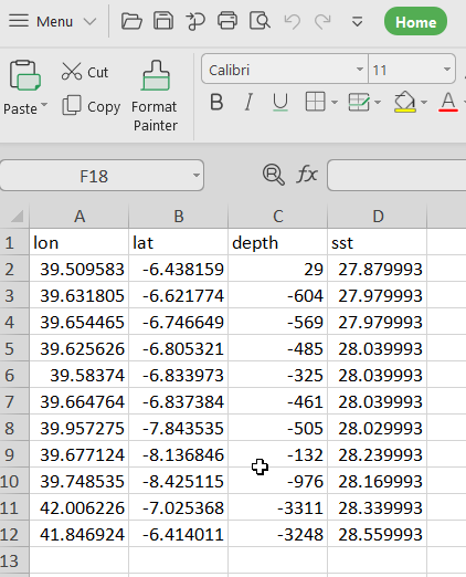
Figure 9.7: Tabulated spatial data
When you face such a case, then st_read() function is out of space. You will need first to import the data using an appropriate read.csv() function first.
        lon       lat depth      sst
1  39.50958 -6.438159    29 27.87999
2  39.63180 -6.621774  -604 27.97999
3  39.65447 -6.746649  -569 27.97999
4  39.62563 -6.805321  -485 28.03999
5  39.58374 -6.833973  -325 28.03999
6  39.66476 -6.837384  -461 28.03999
7  39.95728 -7.843535  -505 28.02999
8  39.67712 -8.136846  -132 28.23999
9  39.74853 -8.425115  -976 28.16999
10 42.00623 -7.025368 -3311 28.33999
11 41.84692 -6.414011 -3248 28.55999
Once the file is in our R session, we can then convert it to simple feature using the longitude and latitude information contained in the file as the chunk below highlight
Simple feature collection with 11 features and 2 fields
geometry type:  POINT
dimension:      XY
bbox:           xmin: 39.50958 ymin: -8.425115 xmax: 42.00623 ymax: -6.414011
CRS:            NA
First 10 features:
   depth      sst                   geometry
1     29 27.87999 POINT (39.50958 -6.438159)
2   -604 27.97999  POINT (39.6318 -6.621774)
3   -569 27.97999 POINT (39.65447 -6.746649)
4   -485 28.03999 POINT (39.62563 -6.805321)
5   -325 28.03999 POINT (39.58374 -6.833973)
6   -461 28.03999 POINT (39.66476 -6.837384)
7   -505 28.02999 POINT (39.95728 -7.843535)
8   -132 28.23999 POINT (39.67712 -8.136846)
9   -976 28.16999 POINT (39.74853 -8.425115)
10 -3311 28.33999 POINT (42.00623 -7.025368)
When printed, the report provide the necesary information, however,the coordinate system is missing. That is true, when we import data from table and convert them to simple feature, we also need to define the coordinate system. There is the function st_set_crs(), which can be used in a to define the CRS. Because of the complexity of the CRS, for this case, we borrow from the existing file and use it to define the missing CRS in our file.
## borrow the coordinate from existing simple feature
crs = sf::st_crs(sampling.points)

## parse the borrowed crs to define the missing CRS in the file
stations.sf.wgs84 = stations.sf %>%
  sf::st_set_crs(crs)

stations.sf.wgs84
Simple feature collection with 11 features and 2 fields
geometry type: POINT
dimension: XY
bbox: xmin: 39.50958 ymin: -8.425115 xmax: 42.00623 ymax: -6.414011
geographic CRS: WGS 84
First 10 features:
depth sst geometry
1 29 27.87999 POINT (39.50958 -6.438159)
2 -604 27.97999 POINT (39.6318 -6.621774)
3 -569 27.97999 POINT (39.65447 -6.746649)
4 -485 28.03999 POINT (39.62563 -6.805321)
5 -325 28.03999 POINT (39.58374 -6.833973)
6 -461 28.03999 POINT (39.66476 -6.837384)
7 -505 28.02999 POINT (39.95728 -7.843535)
8 -132 28.23999 POINT (39.67712 -8.136846)
9 -976 28.16999 POINT (39.74853 -8.425115)
10 -3311 28.33999 POINT (42.00623 -7.025368)We can also use the EPSG code, which is a a four–five digit number that represent Coordinate Reference System, for instance the EPSG code for World Geodetic System of 1984 is 4326.
Simple feature collection with 11 features and 2 fields
geometry type:  POINT
dimension:      XY
bbox:           xmin: 39.50958 ymin: -8.425115 xmax: 42.00623 ymax: -6.414011
geographic CRS: WGS 84
First 10 features:
   depth      sst                   geometry
1     29 27.87999 POINT (39.50958 -6.438159)
2   -604 27.97999  POINT (39.6318 -6.621774)
3   -569 27.97999 POINT (39.65447 -6.746649)
4   -485 28.03999 POINT (39.62563 -6.805321)
5   -325 28.03999 POINT (39.58374 -6.833973)
6   -461 28.03999 POINT (39.66476 -6.837384)
7   -505 28.02999 POINT (39.95728 -7.843535)
8   -132 28.23999 POINT (39.67712 -8.136846)
9   -976 28.16999 POINT (39.74853 -8.425115)
10 -3311 28.33999 POINT (42.00623 -7.025368)Once we have created a simple feature, define the CRS, We can go ahead and plot the stations.sf.wgs84 shown in figure 9.8.
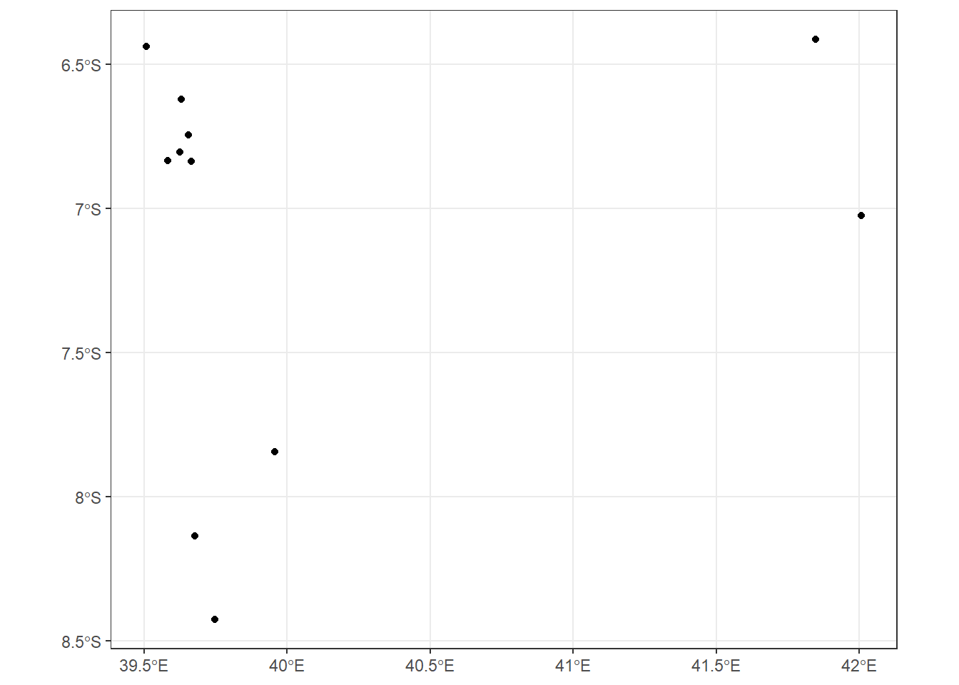
Figure 9.8: Sampling points
9.5.2 Geographic Coordinate Sytem
In GIS, every dataset is associated with a coordinate system, which is a system for representing the locations of different geographic features and different measurements. There are two main types of coordinate systems: geographic coordinate systems (GCS) and projected coordination systems. One example of GCS is using latitude-longitude, and one example of a projected coordination system is the transverse Mercator system. Whereas GCS uses a three-dimensional spherical surface, the projected coordination system uses two dimensions for representing spatial data.
9.5.2.1 Changing projection system
Data is used in GCS to different the position of the spheroid in relation to the center of the earth; a very commonly used GCS is WGS 84. We may sometimes required to change coordinate system, let us say we want to change from GCS to UTM. That is simple using a st_transform and parse crs of intent. For this case, my data is found in UTM zone 37 south and the EPSG code specific for that zone is 32737
Simple feature collection with 11 features and 2 fields
geometry type:  POINT
dimension:      XY
bbox:           xmin: 556349.3 ymin: 9068626 xmax: 832171.7 ymax: 9290155
projected CRS:  WGS 84 / UTM zone 37S
First 10 features:
   depth      sst                 geometry
1     29 27.87999 POINT (556349.3 9288332)
2   -604 27.97999 POINT (569839.6 9268018)
3   -569 27.97999 POINT (572326.2 9254210)
4   -485 28.03999 POINT (569130.6 9247727)
5   -325 28.03999 POINT (564498.3 9244566)
6   -461 28.03999 POINT (573450.6 9244177)
7   -505 28.02999 POINT (605535.5 9132879)
8   -132 28.23999 POINT (574595.1 9100511)
9   -976 28.16999 POINT (582402.5 9068626)
10 -3311 28.33999 POINT (832171.7 9222380)
9.6 Summary
In this tutorial, we learned about the basics of GIS and learned particularly how vector data is stored in R. We learned to import point data from an Excel file and how to map in R. We used the ggplot2 package of R to accomplish this task along with various options for plotting these. We learned to use the st_read() function of the sf package for importing shapefile containing different vector classes. In this tutorial, we also learned how to transform geographical coordinate system from spherical longitude and latitude to flat surface presented in UTM measured in meters.
9.7 Questions
After completing this tutorial, readers should be comfortable to answer the following questions
- What are two main spatial data classes used to represent feature in GIS?
- How can you distinguish vector from raster data format used to represent features in GIS?
- Why we need Cooridnate systems?
- Distinguish between geographic coordinate system and projected cooridnate system
9.8 FUrther readings
When going through vector data manipulation in R, we have just touched the surface of what could be possible using R. We will cover other data manipulation techniques as we step on through proceeding tutorial. But if you want to have a more in-depth discussion about these topics, you can have a look at the book Learning R for Geospatial Analysis by Michael Dorman and An Introduction to R for Spatial Analysis and Mapping by Brunsdon and Comber.
References
Lovelace, Robin, Jakub Nowosad, and Jannes Muenchow. 2019. Geocomputation with R. CRC Press.