Chapter 3 Understanding Data in R
In tutorial 1, we got a glimpse of GIS and the software used in this field. In this tutorial we focus on lower level data types that R handles. This includes understanding how to manage the numeric type (integer vs. double) and strings. The series of data called vectors and tabular format of data storage called data frames. But before we move further, let’s us clean our working environment by clicking a combination of Ctrl+L. Clearing the workspace is always recommended before working on a new R project to avoid name conflicts with provious projects. We can also clear all figures using graphics.off() function. It is a good code practice that a new R project start with the code in the chunk below:
3.1 Data Types
R language is a flexible language that allows to work with different kind of data format (R Core Team 2020). This include integer, numeric, character, complex, dates and logical. The default data type or class in R is double precision—numeric. In a nutshell, R treats all kind of data into five categories but we deal with only four in this book. Before proceeding, we need to clear the workspace by typing rm(list = ls()) after the prompt in the in a console.
3.2 Vectors
Ofen times we want to store a set of numbers in once place. One way to do this is using the vectors in R. Vector is the most basic data structure in R. It is a sequence of elements of the same data type. if the elements are of different data types, they be coerced to a commontype that can accommodate all the elelements. Vector are generally created using the c() function widely called concatenate, though depending on the type vector being created, other method.
Vectors store several numbers– a set of numbers in one container. let us look on the example below
id = c(1,2,3,4,5)
people = c(158,659,782,659,759)
street = c("Dege", "Mchikichini", "Mwembe Mdogo", "Mwongozo",  "Cheka")
Notice that the c() function, which is short for concatenate wraps the list of numbers. The c() function combines all numbers together into one container. Notice also that all the individual numbers are separated with a comma. The comma is referred to an an item-delimiter. It allows R to hold each of the numbers separately. This is vital as without the item-delimiter, R will treat a vector as one big, unseperated number.
3.2.1 Numeric Vector
The numeric class holds the set of real numbers — decimal place numbers. The numeric class is more general than the integer class, and inclused the integer numbers. We create a numeric vector using a c() function but you can use any function that creates a sequence of numbers. These could be any number (whole or decimal number). You can check if the data is integer with is.integer()
[1] TRUE3.2.2 Integer vector
Unlike numeric, integer values do not have decimal places. They are commonly used for counting or indexing. Creating an integer vector is similar to numeric vector except that we need to instruct R to treat the data as integer and not numeric or double. To command R creating integer, we specify a suffix L to an element
[1] TRUE[1] "integer"You can check if the data is integer with is.integer() and can convert numeric value to an integer with as.integer()
[1] FALSEYou can query the class of the object with the class() to know the class of the object
[1] "numeric"Although the object bb is integer as confirmed with as.integer() function, the class() ouput the answer as numeric. This is because the defaul type of number in r is numeric. However, you can use the function as.integer() to convert numeric value to integer
[1] "integer"3.2.3 Character vector
In programming terms, we usually call text as string. This often are text data like names. A character vector may contain a single character , a word or a group of words. The elements must be enclosed with a single or double quotations mark.
[1] TRUE[1] "character"We can be sure whether the object is a string with is.character() or check the class of the object with class().
[1] "character"3.2.4 Factor vector
These are strings from finite set of values. For example, we might wish to store a variable that records gender of people. You can check if the data is factor with is.factor() and use as.factor() to convert string to factor
[1] "factor"Often times we need to know the possible groups that are in the factor data. This can be achieved with the levels() function
[1] "Female" "Male" NULLOften we wish to take a continuous numerical vector and transform it into a factor. The function cut() takes a vector of numerical data and creates a factor based on your give cut-points. Let us make a fictional income of 508 people with rnorm() function.
income = rnorm(n = 508, mean = 500, sd = 80)
hist(income, col = "green", main = "", las = 1, xlab = "Individual Income")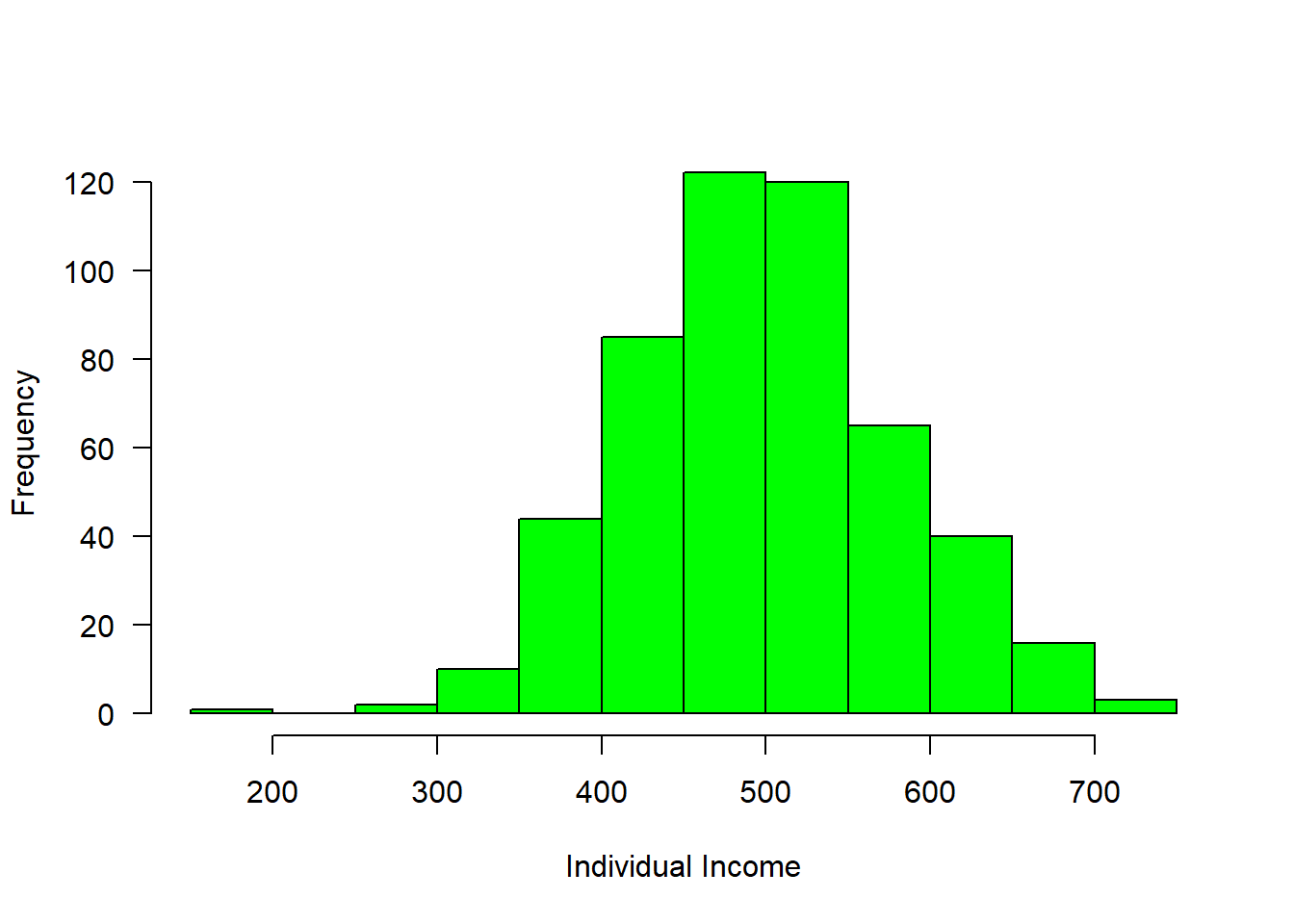
Figure 3.1: Income distribution
We can now breaks the distribution into groups and make a simple plot as shown in figure 3.2, where those with income less than 400 were about 50, followed with a group with income range between 400 and 500 of about 200 and 250 people receive income above 500
group = cut(income, breaks = c(300,400,500,800),
            labels = c("Below 400", "400-500", "Above 500"))
is.factor(group)
[1] TRUE[1] "Below 400" "400-500" "Above 500"barplot(table(group), las = 1, horiz = FALSE, col = c("blue", "red", "blue"), ylab = "Frequency", xlab = "Group of Income")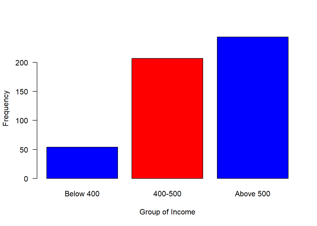
Figure 3.2: Barplot of grouped income
3.2.5 Logical Vector
A vector of logical values will either contain TRUE or FALSE or both. This is a special case of a factor that can only take on the values TRUE and FALSE. R is case-sensitive, therefore you must always capitalize TRUE and FALSE in function in R.
[1] TRUE[1] "logical"3.2.6 Date and Time
Date and time are also treated as vector in R
[1] "2021-01-01" "2021-01-07" "2021-01-13"
[4] "2021-01-19" "2021-01-25"
3.2.7 Indexing the element
One advantage of vector is that you can extract individual element in the vector object by indexing, which is accomplished using the square bracket as illustrated below.
[1] 5[1] 759[1] "Cheka"Apart from extracting single element, indexing allows to extract a range of element in a vector. This is extremely important because it allows to subset a portion of data in a vector. A colon operator is used to extract a range of data
[1] "Mchikichini" "Mwembe Mdogo" "Mwongozo" 3.2.8 Adding and Replacing an element in a vector
It is possible to add element of an axisting vecor. Here ia an example
Sometimes you may need to replace an element from a vector, this can be achieved with indexing
3.2.9 Number of elements in a vector
Sometimes you may have a long vector and want to know the numbers of elements in the object. R has length() function that allows you to query the vector and print the answer
[1] 63.2.10 Generating sequence of vectors Numbers
There are few R operators that are designed for creating vecor of non-random numbers. These functions provide multiple ways for generating sequences of numbers
The colon : operator, explicitly generate regular sequence of numbers between the lower and upper boundary numbers specified. For example, generating number beween 0 and 10, we simply write;
[1] 0 1 2 3 4 5 6 7 8 9 10However, if you want to generate a vector of sequence number with specified interval, let say we want to generate number between 0 and 10 with interval of 2, then the seq() function is used
[1] 0 2 4 6 8 10unlike the seq() function and : operator that works with numbers, the rep() function generate sequence of repeated numbers or strings to create a vector
[1] 3 3 3 3[1] "Station1" "Station1" "Station1" "Station1"The rep() function allows to parse each and times arguments. The each argument allows creation of vector that that repeat each element in a vector according to specified number.
[1] "January" "January" "January" "March"   "March"
[6] "March"   "May"     "May"     "May"
But the times argument repeat the whole vector to specfied times
[1] "January" "March"   "May"     "January" "March"
[6] "May"     "January" "March"   "May"
3.2.11 Generating vector of normal distribution
The central limit theorem that ensure the data is normal distributed is well known to statistician. R has a rnorm() function which makes vector of normal distributed values. For example to generate a vector of 40 sea surface temperature values from a normal distribution with a mean of 25, and standard deviation of 1.58, we simply type this expression in console;
 [1] 23.53896 25.41704 29.05143 21.88331 27.80019
 [6] 25.32484 26.53750 24.83934 21.90669 26.40397
[11] 27.10452 24.54453 22.89453 22.55194 25.47323
[16] 24.43212 25.06017 24.42305 25.67659 25.61061
[21] 21.57773 22.59587 25.81376 25.55776 27.67474
[26] 26.95813 23.90916 27.80628 26.68281 24.84558
[31] 26.03314 23.99131 22.24853 26.00972 24.28766
[36] 25.71115 23.96549 23.49277 27.59002 26.28672
3.2.12 Rounding off numbers
There are many ways of rounding off numerical number to the nearest integers or specify the number of decimal places. the code block below illustrate the common way to round off:
 [1] 0.82 0.65 0.54 0.52 0.64 0.74 0.60 0.59 0.42 1.02
[11] 0.73 0.49 0.77 0.74 0.49 0.59 0.36 0.63 0.63 0.73
3.3 Data Frame
data.frame is very much like a simple Excel spreadsheet where each column represents a variable type and each row represent observations. A data frame is the most common way of storing data in R and, generally, is the data structure most often used for data analyses. A data frame is a list of equal–length vectors with rows as records and columns as variables. This makes data frames unique in data storing as it can store different classes of objects in each column (i.e. numeric, character, factor, logic, etc). In this section, we will create data frames and add attributes to data frames.
3.3.1 Creating data frames
Perhaps the easiest way to create a data frame is to parse vectors in a data.frame() function. For instance, in this case we create a simple data frame dt and assess its internal structure
# create vectors
Name  = c('Bob','Jeff','Mary')
Score = c(90, 75, 92)
Grade = c("A", "B", "A")

## use the vectors to make a data frame
dt = data.frame(Name, Score, Grade)

## assess the internal structure
str(dt)
'data.frame': 3 obs. of 3 variables:
$ Name : Factor w/ 3 levels "Bob","Jeff","Mary": 1 2 3
$ Score: num 90 75 92
$ Grade: Factor w/ 2 levels "A","B": 1 2 1Note how Variable Name in dt was converted to a column of factors . This is because there is a default setting in data.frame() that converts character columns to factors . We can turn this off by setting the stringsAsFactors = FALSE argument:
## use the vectors to make a data frame
df = data.frame(Name, Score, Grade, stringsAsFactors = FALSE)
df %>% str()
'data.frame': 3 obs. of 3 variables:
$ Name : chr "Bob" "Jeff" "Mary"
$ Score: num 90 75 92
$ Grade: chr "A" "B" "A"Now the variable Name is of character class in the data frame. The inherited problem of data frame to convert character columns into a factor is resolved by introduction f advanced data frames called tibble (Müller and Wickham 2020), which provides sticker checking and better formating than the traditional data.frame.
## use the vectors to make a tibble
tb = tibble(Name, Score, Grade)
## check the internal structure of the tibble
tb%>% glimpse()
Rows: 3
Columns: 3
$ Name <chr> "Bob", "Jeff", "Mary"
$ Score <dbl> 90, 75, 92
$ Grade <chr> "A", "B", "A"Table 3.1 show the the data frame created by fusing the two vectors together.
| Name | Score | Grade |
|---|---|---|
| Bob | 90 | A |
| Jeff | 75 | B |
| Mary | 92 | A |
Because the columns have meaning and we have given them column names, it is desirable to want to access an element by the name of the column as opposed to the column number.In large Excel spreadsheets I often get annoyed trying to remember which column something was. The $sign and []are used in R to select variable from the data frame.
[1] Bob  Jeff Mary
Levels: Bob Jeff Mary[1] Bob Jeff Mary
Levels: Bob Jeff Mary[1] 90 75 92[1] 90 75 92R has build in dataset that we can use for illustration. For example, Longley (1967) created a longley dataset, which is data frame with 7 economic variables observed every year from 1947 ti 1962 (Table 3.2). We can add the data in the workspace with data() function
data(longley)

longley %>%
  kableExtra::kable(caption = "Longleys' Economic dataset",
                    align = "c", row.names = F) %>%
kableExtra::column_spec(1:7, width = "3cm")| GNP.deflator | GNP | Unemployed | Armed.Forces | Population | Year | Employed |
|---|---|---|---|---|---|---|
| 83.0 | 234.289 | 235.6 | 159.0 | 107.608 | 1947 | 60.323 |
| 88.5 | 259.426 | 232.5 | 145.6 | 108.632 | 1948 | 61.122 |
| 88.2 | 258.054 | 368.2 | 161.6 | 109.773 | 1949 | 60.171 |
| 89.5 | 284.599 | 335.1 | 165.0 | 110.929 | 1950 | 61.187 |
| 96.2 | 328.975 | 209.9 | 309.9 | 112.075 | 1951 | 63.221 |
| 98.1 | 346.999 | 193.2 | 359.4 | 113.270 | 1952 | 63.639 |
| 99.0 | 365.385 | 187.0 | 354.7 | 115.094 | 1953 | 64.989 |
| 100.0 | 363.112 | 357.8 | 335.0 | 116.219 | 1954 | 63.761 |
| 101.2 | 397.469 | 290.4 | 304.8 | 117.388 | 1955 | 66.019 |
| 104.6 | 419.180 | 282.2 | 285.7 | 118.734 | 1956 | 67.857 |
| 108.4 | 442.769 | 293.6 | 279.8 | 120.445 | 1957 | 68.169 |
| 110.8 | 444.546 | 468.1 | 263.7 | 121.950 | 1958 | 66.513 |
| 112.6 | 482.704 | 381.3 | 255.2 | 123.366 | 1959 | 68.655 |
| 114.2 | 502.601 | 393.1 | 251.4 | 125.368 | 1960 | 69.564 |
| 115.7 | 518.173 | 480.6 | 257.2 | 127.852 | 1961 | 69.331 |
| 116.9 | 554.894 | 400.7 | 282.7 | 130.081 | 1962 | 70.551 |
Sometimes you may need to create set of values and store them in vectors, then combine the vectors into a data frame. Let us see how this can be done. First create three vectors. One contains id for ten individuals, the second vector hold the time each individual signed in the attendane book and the third vector is the distance of each individual from office. We can concatenate the set of values to make vectors.
id  = c(1,2,3,4,5,6,7,8,9,10)

time = lubridate::ymd_hms(c("2018-11-20 06:35:25 EAT", "2018-11-20 06:52:05 EAT",
                 "2018-11-20 07:08:45 EAT", "2018-11-20 07:25:25 EAT",
                 "2018-11-20 07:42:05 EAT", "2018-11-20 07:58:45 EAT",
                 "2018-11-20 08:15:25 EAT", "2018-11-20 08:32:05 EAT",
                 "2018-11-20 08:48:45 EAT", "2018-11-20 09:05:25 EAT"), tz = "")

distance = c(20, 85, 45, 69, 42,  52, 6, 45, 36, 7)
Once we have the vectors that have the same length dimension, we can use the function data.frame() to combine the the three vectors into one data frame shown in table 3.3
| IDs | Time | Distance |
|---|---|---|
| 1 | 2018-11-20 06:35:25 | 20 |
| 2 | 2018-11-20 06:52:05 | 85 |
| 3 | 2018-11-20 07:08:45 | 45 |
| 4 | 2018-11-20 07:25:25 | 69 |
| 5 | 2018-11-20 07:42:05 | 42 |
| 6 | 2018-11-20 07:58:45 | 52 |
| 7 | 2018-11-20 08:15:25 | 6 |
| 8 | 2018-11-20 08:32:05 | 45 |
| 9 | 2018-11-20 08:48:45 | 36 |
| 10 | 2018-11-20 09:05:25 | 7 |
3.4 Matrix
A matrix is defined as a collection of data elements arranged in a two–dimensional rectangular layout. R is very strictly when you make up a matrix as it must be with equal dimension—all columns in a matrix must be of the same length. Unlike data frame and list that can store numeric or character.etc in columns, matrix columns must be numeric or characters in a matrix file.
3.4.1 Creating Matrices
The base R has a matrix() function that construct matrices column–wise. In other language, element in matrix are entered starting from the upper left corner and running down the columns. Therefore, one should take serious note of specifying the value to fill in a matrix and the number of rows and columns when using the matrix() function.For example in the code block below, we create an imaginary month sst value for five years and obtain an atomic vector of 60 observation.
Once we have the atomic vector of sst value, we can convert it to matrix with the matrix() function. We put the observation as rows—months and the columns as years. Therefore, we have 12 rows and 5 years and the product of number of months and years we get 60—equivalent to our sst atomic vector we just created above.
We then check whether we got the matrix with is.matrix() function
[1] FALSE[1] TRUE [1] 24.12749 27.48300 24.59168 24.84240 20.26587
[6] 23.02858 22.43177 30.98097 28.34107 23.57099
[11] 25.93713 22.69718 25.63378 21.60883 17.71580
[16] 27.87434 25.45653 24.72419 25.02352 25.05497
[21] 26.12613 25.58128 25.03653 23.32987 25.79478
[26] 23.22245 21.21783 23.63734 26.58929 25.76394
[31] 25.85704 26.88392 26.31193 20.80500 26.28160
[36] 26.09082 21.99118 26.15753 24.70482 30.74588
[41] 22.86493 24.05142 24.90224 20.61996 28.10089
[46] 25.76837 24.73541 26.83625 20.82912 26.17858
[51] 23.55351 26.71082 21.55226 23.82109 28.73656
[56] 21.09010 21.98741 23.24176 23.50238 21.40391We can check whether the dimension we just defined while creating this matrix is correct. This is done with the dim() function from base R.
[1] 12 5If you have large vector and you you want the matrix() function to figure out the number of columns, you simply define the nrow and tell the function that you do not want those element arranged by rows —i.e you want them in column-wise. That is done by parsing the argument byrow = FALSE inside the matrixt() function.
3.4.2 Adding attributes to Matrices
Often times you may need to add additional attributes to the maxtrix—observation names, variable names and comments in the matrix.
We can add columns, which are years from 2014 to 2018
          2014     2015     2016     2017     2018
 [1,] 24.12749 25.63378 25.79478 21.99118 20.82912
 [2,] 27.48300 21.60883 23.22245 26.15753 26.17858
 [3,] 24.59168 17.71580 21.21783 24.70482 23.55351
 [4,] 24.84240 27.87434 23.63734 30.74588 26.71082
 [5,] 20.26587 25.45653 26.58929 22.86493 21.55226
 [6,] 23.02858 24.72419 25.76394 24.05142 23.82109
 [7,] 22.43177 25.02352 25.85704 24.90224 28.73656
 [8,] 30.98097 25.05497 26.88392 20.61996 21.09010
 [9,] 28.34107 26.12613 26.31193 28.10089 21.98741
[10,] 23.57099 25.58128 20.80500 25.76837 23.24176
[11,] 25.93713 25.03653 26.28160 24.73541 23.50238
[12,] 22.69718 23.32987 26.09082 26.83625 21.40391
and add the month for rows, which is January to December. Now the matrix has names for the rows—records and for columns—variables
months = seq(from = lubridate::dmy(010115), to = lubridate::dmy(311215),
             by = "month") %>% lubridate::month(abbr = TRUE,
                                     label = TRUE)
rownames(sst.matrix) = months
sst.matrix
2014 2015 2016 2017 2018
Jan 24.12749 25.63378 25.79478 21.99118 20.82912
Feb 27.48300 21.60883 23.22245 26.15753 26.17858
Mar 24.59168 17.71580 21.21783 24.70482 23.55351
Apr 24.84240 27.87434 23.63734 30.74588 26.71082
May 20.26587 25.45653 26.58929 22.86493 21.55226
Jun 23.02858 24.72419 25.76394 24.05142 23.82109
Jul 22.43177 25.02352 25.85704 24.90224 28.73656
Aug 30.98097 25.05497 26.88392 20.61996 21.09010
Sep 28.34107 26.12613 26.31193 28.10089 21.98741
Oct 23.57099 25.58128 20.80500 25.76837 23.24176
Nov 25.93713 25.03653 26.28160 24.73541 23.50238
Dec 22.69718 23.32987 26.09082 26.83625 21.403913.5 Arrays
, , 1

         [,1]     [,2]     [,3]     [,4]     [,5]
[1,] 24.12749 24.84240 22.43177 23.57099 25.63378
[2,] 27.48300 20.26587 30.98097 25.93713 21.60883
[3,] 24.59168 23.02858 28.34107 22.69718 17.71580

, , 2

         [,1]     [,2]     [,3]     [,4]     [,5]
[1,] 27.87434 25.02352 25.58128 25.79478 23.63734
[2,] 25.45653 25.05497 25.03653 23.22245 26.58929
[3,] 24.72419 26.12613 23.32987 21.21783 25.76394

, , 3

         [,1]     [,2]     [,3]     [,4]     [,5]
[1,] 25.85704 20.80500 21.99118 30.74588 24.90224
[2,] 26.88392 26.28160 26.15753 22.86493 20.61996
[3,] 26.31193 26.09082 24.70482 24.05142 28.10089

, , 4

         [,1]     [,2]     [,3]     [,4]     [,5]
[1,] 25.76837 20.82912 26.71082 28.73656 23.24176
[2,] 24.73541 26.17858 21.55226 21.09010 23.50238
[3,] 26.83625 23.55351 23.82109 21.98741 21.40391
This can be done with the indexing. For example, in the sst.matrix we just create, it has twelve rows representing monthly average and five columns representing years. We then obtain data for the six year and we want to add it into the matrix. Simply done with indexing
     Jan      Feb      Mar      Apr      May      Jun
20.82912 26.17858 23.55351 26.71082 21.55226 23.82109
     Jul      Aug      Sep      Oct      Nov      Dec
28.73656 21.09010 21.98741 23.24176 23.50238 21.40391
3.6 Dealing with Misiing Values
Just as we can assign numbers, strings, list to a variable, we can also assign nothing to an object, or an empty value to a variable. IN R, an empty object is defined with NULL. Assigning a value oof NULL to an object is one way to reset it to its original, empty state. You might do this when you wanto to pre–allocate an object without any value, especially when you iterate the process and you want the outputs to be stored in the empty object.
You can check whether the object is an empty with the is.null() function, which return a logical ouputs indicating whther is TRUE or FALSE
[1] TRUEYou can also check for NULL in an if satement as well, as highlighted in the following example;
if (is.null(sst.container)){
  print("The object is empty and hence you can use to store looped outputs!!!")
}
[1] "The object is empty and hence you can use to store looped outputs!!!"And empty element (value) in object is represented with NA in R, and it is the absence of value in an object or variable.
[1] 26.78 25.98 NA 24.58 NATo identify missing values in a vector in R, use the is.na() function, which returns a logical vector with TRUE of the corresponding element(s) with missing value
[1] FALSE FALSE TRUE FALSE TRUEand computing statistics of the variable with NA always will give out the NA ouputs
[1] NA[1] NA[1] NA NAHowever, we can exclude missing value in these mathematical operations by parsing , na.rm = TRUE argument
[1] 25.78[1] 1.113553[1] 24.58 26.78you can also exclude the element with NA value using the `na.omit()
[1] 26.78 25.98 24.58
attr(,"na.action")
[1] 3 5
attr(,"class")
[1] "omit"
Finally is a NaN, which is closely related to NA, which is used to assign non-floating numbers. For example when we have the anomaly of sea surface temperature and we are interested to use sqrt() function to reduce the variability of the dataset.
[1] 1.5165751 1.1180340 0.8944272 0.5567764 0.0000000
[6]       NaN
We notice that the sqrt of -0.21 gives us a NaN elements.
References
Longley, J. W. 1967. “An Appraisal of Least-Squares Programs from the Point of View of the User.” Journal of the American Statistical Association, 819–41.
Müller, Kirill, and Hadley Wickham. 2020. Tibble: Simple Data Frames. https://CRAN.R-project.org/package=tibble.
R Core Team. 2020. R: A Language and Environment for Statistical Computing. Vienna, Austria: R Foundation for Statistical Computing. https://www.R-project.org/.