Chapter 6 Visualisation with ggplot`

R provides numerous routines for displaying data as graphics. This chapter introduce the most important graphic functions. The graphics can be modified, printed, embedded in rmarkdown document or exported to be edited with graphic software outside R environment.

There are three major “systems” of making graphs in R. The basic plotting commands in R are quite effective but the commands do not have a way of being combined in easy ways (R Core Team 2018). The simplest function producing a graph of a vector y versus another vector x is plot. First we create two vectors of x and y, where y is the sine of x

x = seq(0,2*pi,pi/10)
y = sin(x)
length(y)

## [1] 21

These two command lines resulted into two vectors with 21 elements each. Since the two vector have the same length dimension, we can use plot() function to produce a 2D graph of y against x. The code produce figure 6.1 with an x-axis ranging from 0 ti 7 and a \(y\)-axis ranging from -1 to +1 and black line overlaid on point.

plot(x,y, type = "b", xlab = "Independent variable", ylab = "Dependent variable")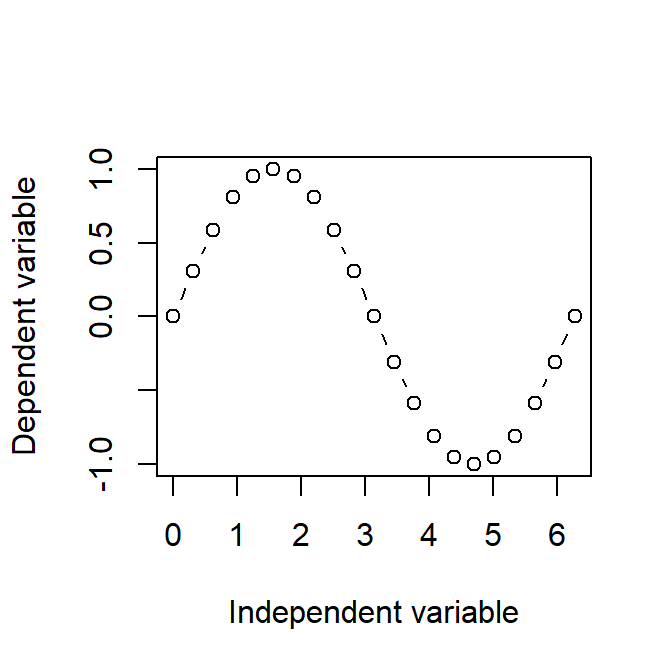

Figure 6.1: Two dimension plot generated with base plot function

We can even combine different plot in one layout with the combination of par() and mfrow() function. For example the code par(mfrow = c(1,3)) tell the computer to create container of one row that can accomodate three plots shown in figure 6.2

par(mfrow = c(1,3))
plot(x,y, type = "p", xlab = "Independent variable", ylab = "Dependent variable")
plot(x,y, type = "l", xlab = "Independent variable", ylab = "Dependent variable")
plot(x,y, type = "b", pch = 8, cex = 2,col = 2 ,xlab = "Independent variable", ylab = "Dependent variable")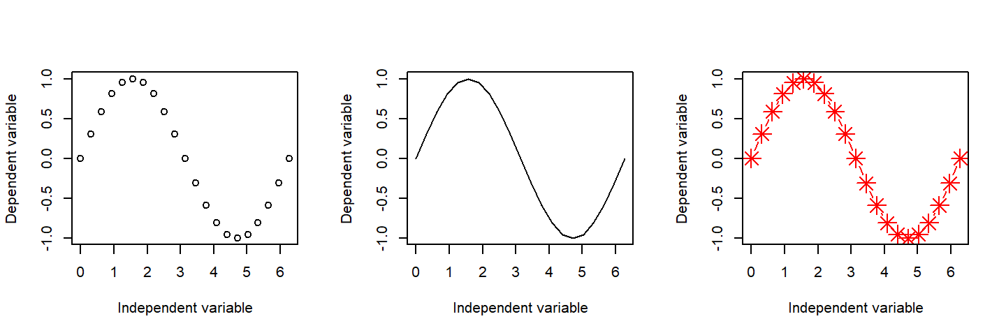

Figure 6.2: Multiple plot in a single layout

Lattice graphics (which the mosaic package uses) makes it possible to create some quite complicated graphs but it is very difficult to do make non-standard graphs (Sarkar 2008). The last package, ggplot2 tries to not anticipate what the user wants to do, but rather provide the mechanisms for pulling together different graphical concepts and the user gets to decide which elements to combine.

The ggplot2 package, created by Hadley Wickham (2016), offers a powerful graphics language for creating elegant and complex plots. Its popularity in the R community has exploded in recent years. Originally based on Leland Wilkinson’s The Grammar of Graphics (2006), ggplot2 allows you to create graphs that represent both univariate and multivariate numerical and categorical data in a straightforward manner. Unfortunate ggplot2 works only with data that are in data frame. If we want to plot the x and y variables we just created, we need to store them in the data frame first for ggplot to draw the graph (Wickham 2017).

We first load the package we need to work with for this chapter into the working directory. I am working a R project and defined the path of the working directory. Make sure you have also specified the path of the working directory. You can check section 2.3 that illustrats how to set a working directory in R.

The default ggplot2 draw a plot with a gray background like the one shown in figure 6.3. We will discuss on how to change and customize plot made with ggplot2, but for now we may focus on the tools of making and draw plot with these package. Once we are familiar with its syntax, we can expand the skills by touching on issue related to creating quality publication plots with ggplot.

y2 = cos(x)

x.ys = data.frame(x,y,y2)

ggplot(data = x.ys, aes(x = x, y = y)) + geom_point() + geom_line()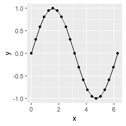

Figure 6.3: Sine plot with ggplot2

Sometimes We may wish to plot two different in one plot. That happen when you have two or more dependent variables and one independent variable. We need to create a second y variable and a cosine of xcan suits well for illustration.

x = seq(0,2*pi,pi/10)
y = sin(x)
y2 = cos(x)

x.ys = data.frame(x,y,y2)

Figure 6.4 show the cosine and sine curves, unfortunately you can not distinguish them because the legend is missing. Here comes the problem inherited with untidy data discussed in chapter 5. Alghout the data is the data frame and ggplot2 can plot them, the data frame is untidy and therefore can not draw the lines with their respective legend. we therefore need to tidy the data and first and replot.

ggplot(data = x.ys) +
  geom_line(aes(x = x, y = y), col = "red", show.legend = TRUE)+
  geom_point(aes(x = x, y = y), col = "red") +
  geom_line(aes(x = x, y = y2), col = "blue", show.legend = TRUE)+
  geom_point(aes(x = x, y = y2), col = "blue")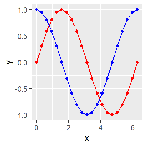

Figure 6.4: Two dependent variables plotted in one independent variable

We first need to transform the data frame from wide to long format with gather() function of tidyr package. Because the x variable is the same for the two ys, we transform the variable y and y2

x.ys.long = x.ys %>% tidyr::gather(key = "ys", value = "values", 2:3)

Once the data is tidy, plotting and define the color makes easy for ggplot to distinguish and label the variables with a legend as shown in figure 6.5

ggplot(data = x.ys.long, aes(x = x, y = values, col = ys))+geom_line() + geom_point()+
  theme(legend.position = "top") +
  scale_colour_manual(values = c("red", "blue"), name = NULL)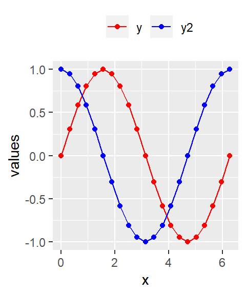

Figure 6.5: Two dependent variables plotted in one independent variable with legend

6.1 Univariate Distributions

Before moving on to more sophisticated visualizations that enable multidimensional investigation, it is important to be able to understand how an individual variable is distributed. Visually understanding the distribution allows us to describe many features of a variable.

6.2 Continuous Variables

A variable is continuous if it can take any of an infinite set of ordered values. There are several different plots that can effectively communicate the different features of continuous variables. Features we are generally interested in include:

Measures of location
Measures of spread
Asymmetry
Outliers
Gaps

Hadley Wickham in his book Elegant Graphics for Data Analysis with ggplot clearly said ggplot2 is designed to act on data frames (Wickham 2016). It is actually hard to just draw three data points and for simple graphs it might be easier to use the base graphing system in R. Fortunate ggplot2 makes plotting easy because of its large number of basic building blocks that, when stacked upon each other, can produce extremely complicated graphs. A full list is available at http://docs.ggplot2.org/current/. In summary, we can break the art of making graph with ggplot2 three main steps.

Understand the type of data you are going to use
Ask yourself what is the major relationship we wish to examine?
Choose the appropriate graph that suits your data.

We will use the audit dataset in table 6.1 to illustrate how to use ggplot2 package to make elegant graphics in R. We chopped this dataset from the rattle package. The audit dataset is an artificially constructed dataset that has some of the characteristics of a true financial audit datase (Maindonald 2012)

Table 6.1: Individual Auditing Infomration
ID	Age	Employment	Education	Marital	Occupation	Income	Gender
6260817	21	Private	College	Absent	Service	119419.36	Male
8511774	50	Private	Associate	Divorced	Repair	87361.20	Male
4527269	36	Private	Bachelor	Married	Support	34606.74	Male
3718723	66	Private	HSgrad	Widowed	Sales	96057.04	Female
4516220	48	Private	Bachelor	Married	Support	113867.76	Female
1158519	45	Private	Vocational	Married	Repair	26717.49	Male
7488134	45	PSLocal	Master	Absent	Professional	54304.38	Female
9717671	53	Consultant	HSgrad	Married	Executive	37678.12	Male
5806158	34	Consultant	College	Divorced	Clerical	201606.08	Female
7219320	25	NA	Bachelor	Married	NA	46429.12	Male

6.3 Graphics with ggplot

6.3.1 Categorical Data

6.3.1.1 Barplot

The ggplot() function only needs to specify the data and aes. Note the unusual use of the plus sign “+” to add the effect of of geom_bar() to ggplot(). Only one variable plays an aesthetic role: workshop. The aes() function sets that role. To produce figure 6.6 you can write the code below:

ggplot(data = audit, 
       aes(x = Education))+
  geom_bar()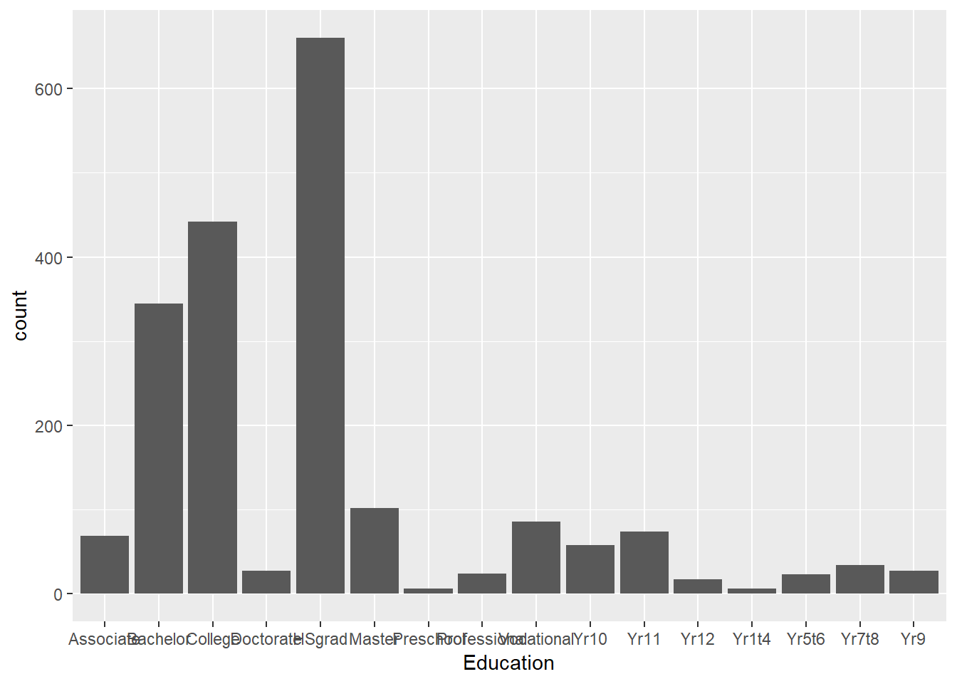

Figure 6.6: Barplot of frequency of people with various education level

Figure 6.6 plot some of the education that are of no interest to us, we can limit the education level by adding a limits function in the scale_x_discrete() function to produce figure 6.7. The code for figure 6.7 is:

ggplot(data = audit, 
       aes(x = Education))+
  geom_bar() +
  scale_x_discrete(limits = c("Preschool", "Vocational", "College","Bachelor", "Master", "Doctorate"))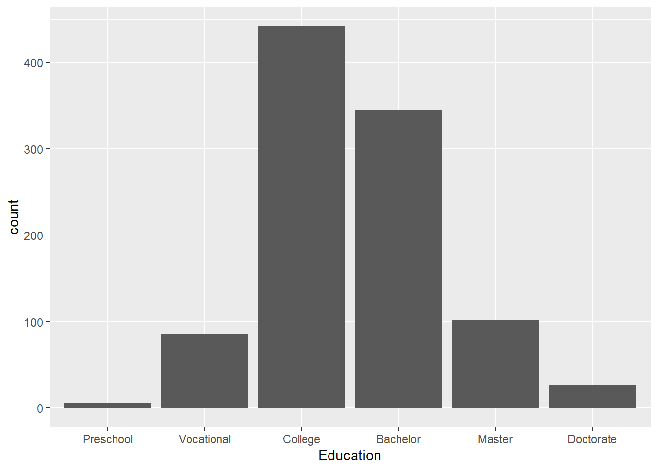

Figure 6.7: Barplot of frequency of people in six education level

If you want to fill the bars with color (Figure 6.8), you can parsethe fill argument in geom_bar().

ggplot(data = audit, 
       aes(x = Education))+
  geom_bar(fill = c("red", "purple", "blue", "green", "maroon", "pink")) +
  scale_x_discrete(limits = c("Preschool", "Vocational", "College","Bachelor", "Master", "Doctorate"))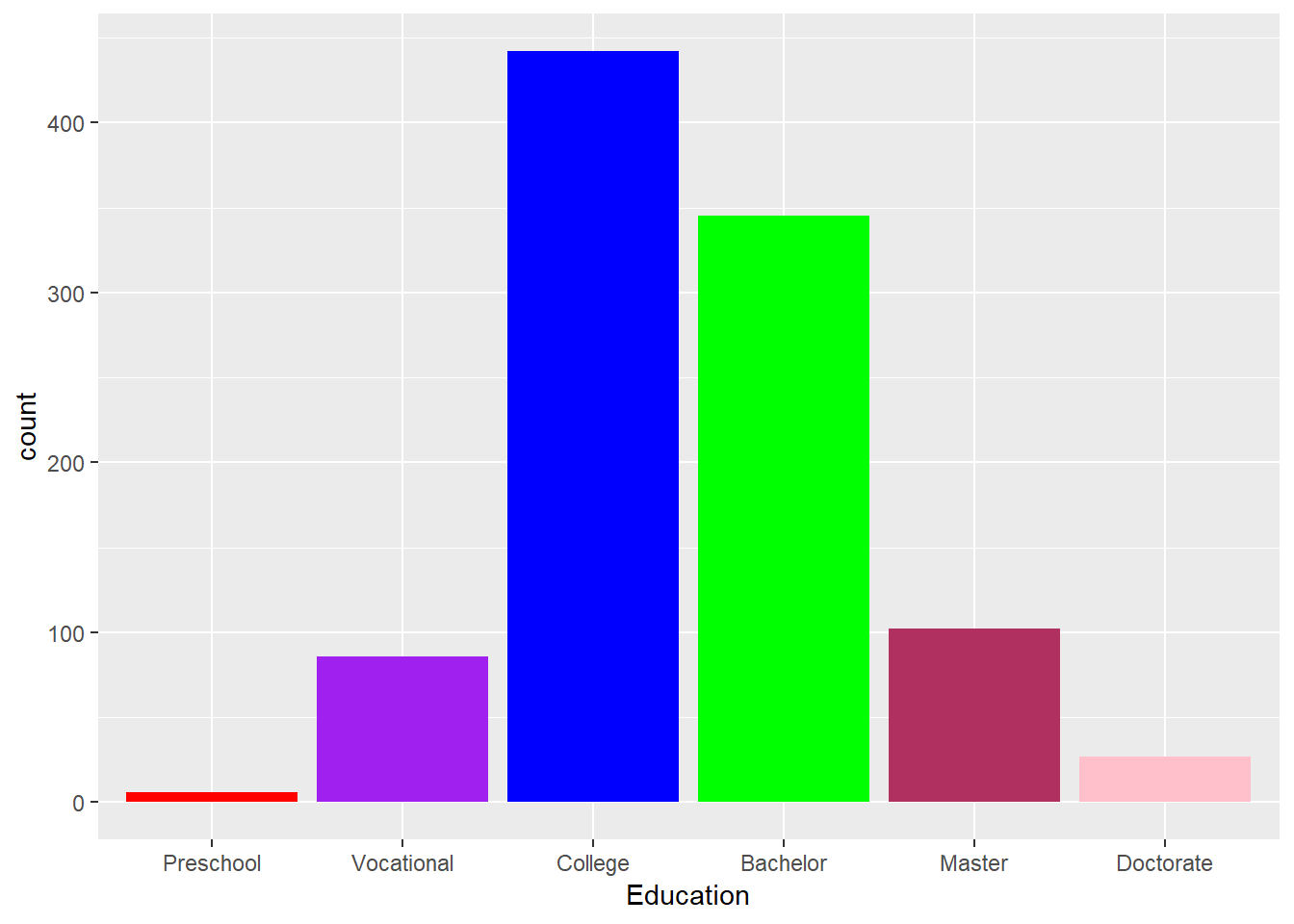

Figure 6.8: Barplot of frequency of people in six education level

The use of color in figure 6.8 was, well, colorful, but it did not add any useful information. However, when displaying bar plots of six education level, the fill argument with Gender very useful. Figure 6.9 I use fill to color the bars by gender and set the “position” to stack.

ggplot(data = audit, 
       aes(x = Education))+
  geom_bar(aes(fill = Gender), position = "stack") +
  scale_x_discrete(limits = c("Preschool", "Vocational", 
                              "College","Bachelor", "Master", "Doctorate"))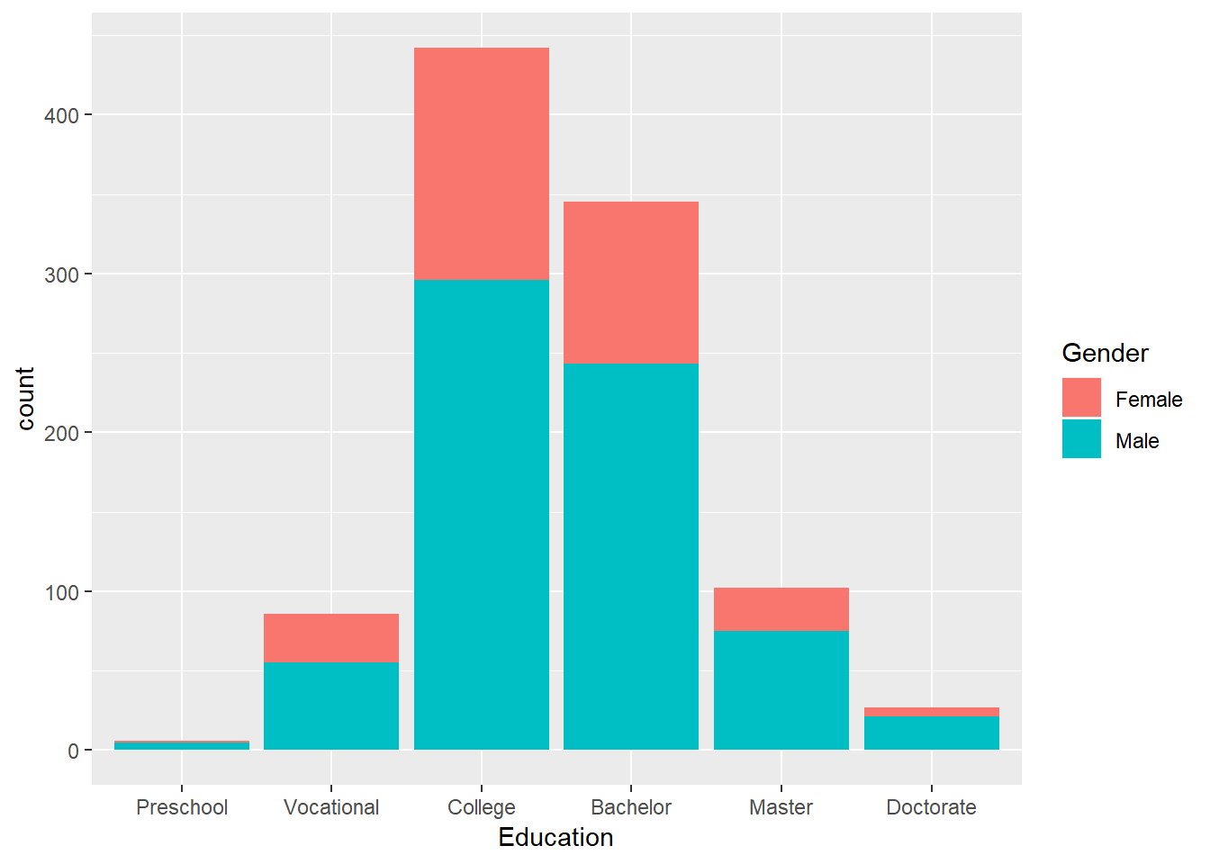

Figure 6.9: Barplot of frequency of people in six education level

Figure 6.10 is similar to figure 6.9, changing only the bar position to be dodge.

ggplot(data = audit, 
       aes(x = Education))+
  geom_bar(aes(fill = Gender), position = "dodge") +
  scale_x_discrete(limits = c("Preschool", "Vocational", 
                              "College","Bachelor", "Master", "Doctorate"))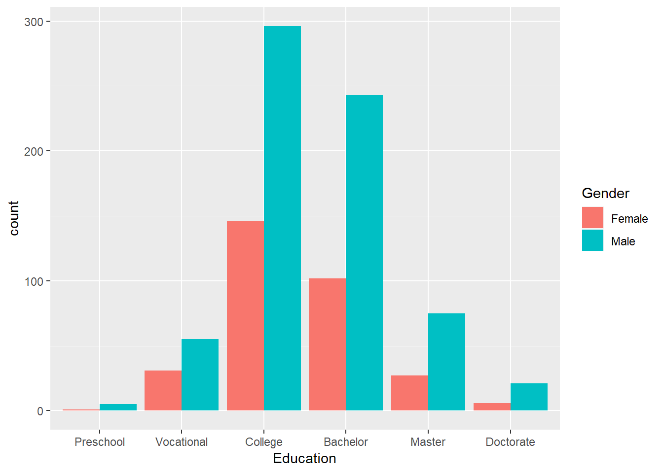

Figure 6.10: Barplot of frequency of people in six education level

6.3.1.2 Pre-summarized Data

The geom_bar() function summarizes data for you. If it is already summarized, you use geom_col() instead. The chunk below summarize the eduction level and then plot the summarized result in figure 6.11.

education = audit %>% 
  filter(Education %in% c("Preschool", "Vocational", 
                              "College","Bachelor", "Master", "Doctorate")) %>%
  group_by(Education) %>%
  summarise(Count = n())

ggplot(data = education, aes(x = Education, y = Count))+geom_col()+
  scale_x_discrete(limits = c("Preschool", "Vocational", 
                              "College","Bachelor", "Master", "Doctorate"))

Figure 6.11: Barplot of frequency of people in six education level

6.3.2 Numerical Data

6.3.2.1 Histograms

Histograms are often overlooked, yet they are a very efficient means for communicating distribution of continuous variables. geom_histogram() is used to make histogram in ggplot2 package. Figure 6.12 was created using the code in the chunk below:

ggplot(data = audit, aes(x = Age)) +
  geom_histogram()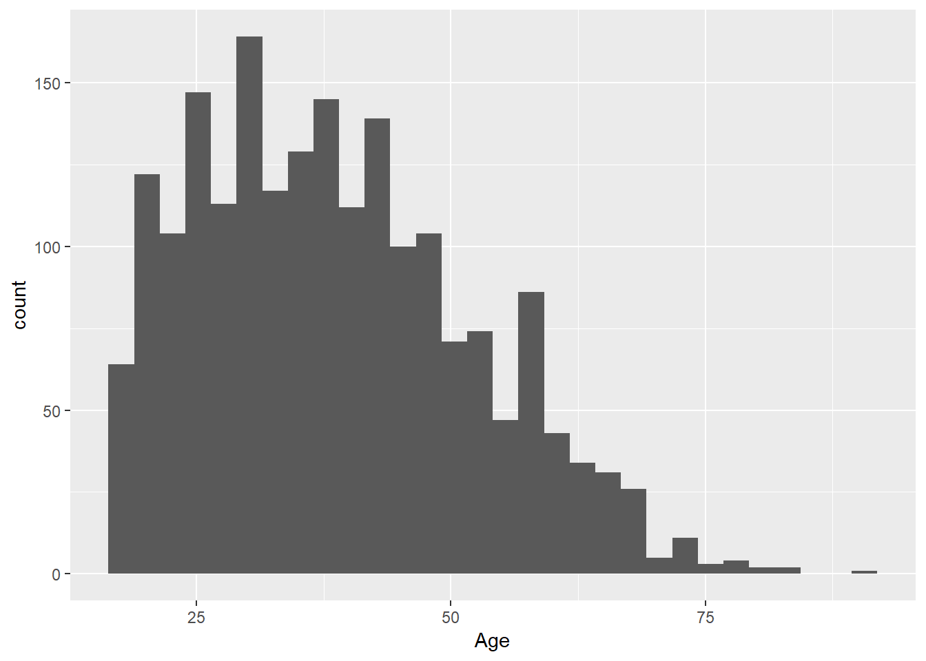

Figure 6.12: Age distribution

labs() function is used in ggplot2 to add annotations in plot as in figure 6.13.

ggplot(data = audit%>% 
  filter(Education %in% c("Preschool", "Vocational", 
                              "College","Bachelor", "Master", "Doctorate")), 
  aes(x = Age)) +
  geom_histogram()+
  labs(x = "Age of Individuals", y = "Number of Individuals", 
       title = "The Age of Individuals audited in US", 
       subtitle = "The audit was done to 2000 individuals aiming to illustrate the auditing")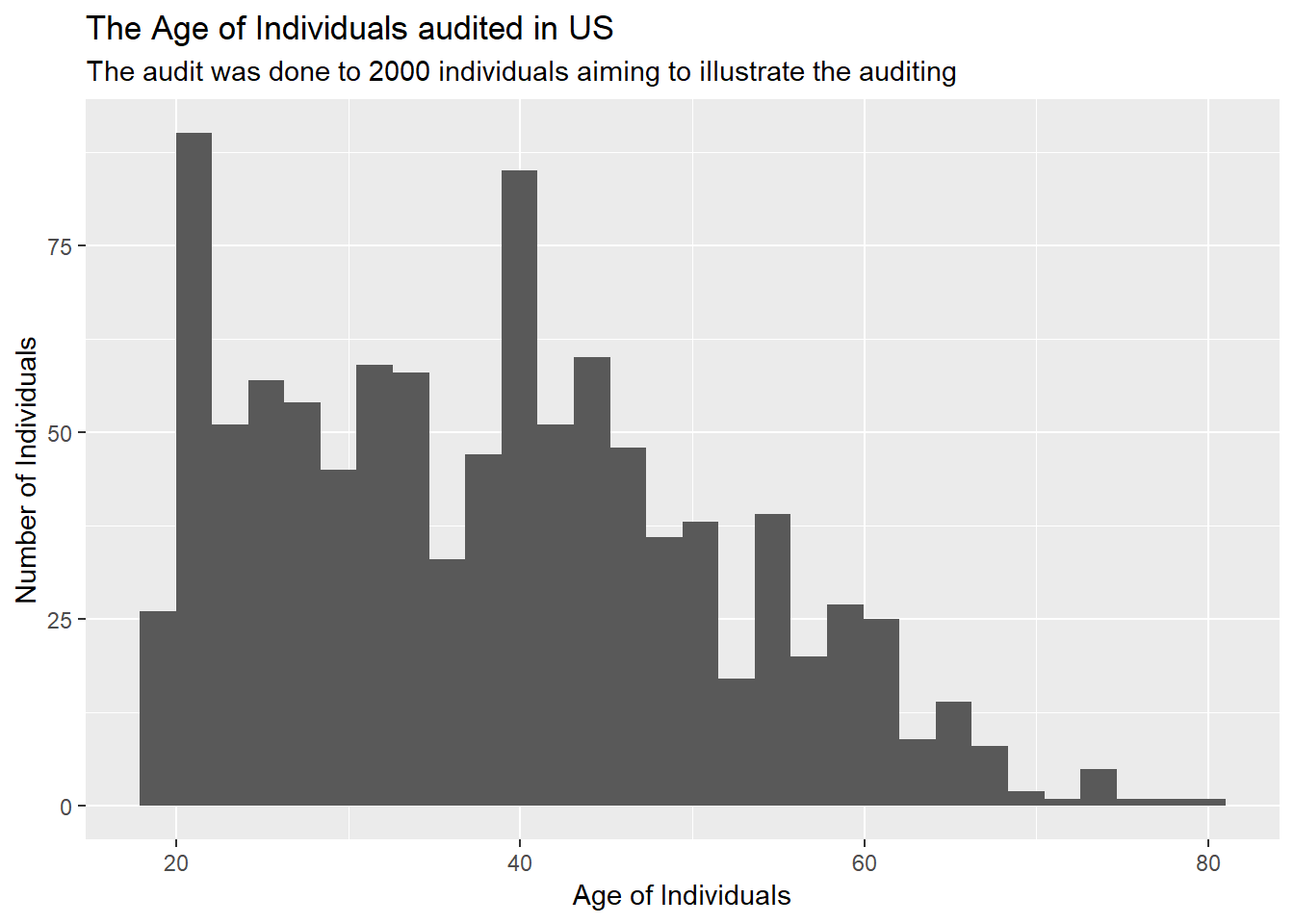

Figure 6.13: Age distribution

facet_wrap() function is used in ggplot2 to make multiple plots in a single layout as illustrated n figure 6.14.

ggplot(data = audit%>% 
  filter(Education %in% c("Preschool", "Vocational", 
                              "College","Bachelor", "Master", "Doctorate")), 
  aes(x = Age)) +
  geom_histogram()+
  labs(x = "Age of Individuals", y = "Number of Individuals") +
  facet_wrap(~Education, scales = "free_y")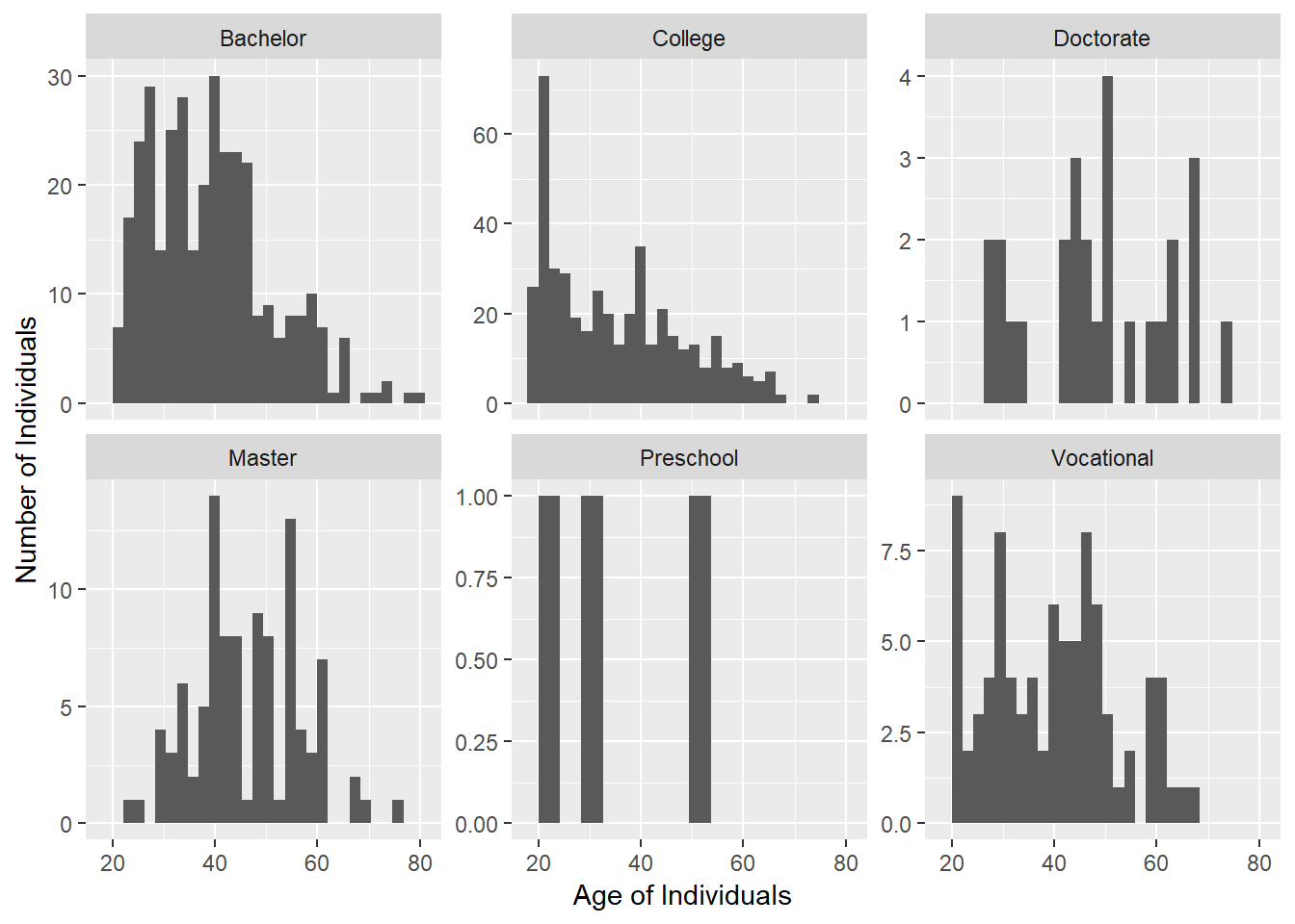

Figure 6.14: Age distribution grouped by education level

References

R Core Team. 2018. R: A Language and Environment for Statistical Computing. Vienna, Austria: R Foundation for Statistical Computing. https://www.R-project.org/.

Sarkar, Deepayan. 2008. Lattice: Multivariate Data Visualization with R. New York: Springer. http://lmdvr.r-forge.r-project.org.

Wickham, Hadley. 2016. Ggplot2: Elegant Graphics for Data Analysis. Springer-Verlag New York. http://ggplot2.org.

Wilkinson, Leland. 2006. The Grammar of Graphics. Springer Science & Business Media.

Wickham, Hadley. 2017. Tidyverse: Easily Install and Load the ’Tidyverse’. https://CRAN.R-project.org/package=tidyverse.

Maindonald, John H. 2012. “Data Mining with Rattle and R: The Art of Excavating Data for Knowledge Discovery by Graham Williams.” International Statistical Review 80 (1). Wiley Online Library: 199–200.