Chapter 3 Importing data with readr
You can lean R with the dataset it comes with when you install it in your machine. But sometimes you want to use the real data you or someone gathered already. One of critical steps for data processing is to import data with special format into R workspace.Data import refers to read data from the working directory into the workspace (Matthew 2018). In this chapter you will learn how to import common files into R. We will only focus on two common types of tabular data storage format—The comma-seprated .csv and excell spreadsheet (.xlsx). In later chapter we will explain how to read other types of data into R.
3.1 Comma-Separated (.csv)
The most commonly format that R like is the comma-separated files. Although Base R provides various functions like read.table(), read.csv(), read.table() and read.csv2() to import data from the local directories into R workspace, for this book we use an read_csv() function from readr. Before we import the data, we need to load the packages that we will use their functions in this chapeter
require(dplyr)
require(readr)
require(lubridate)
require(readxl)
require(haven)
require(ggplot2)
require(kableExtra).csv format in figure 3.1.
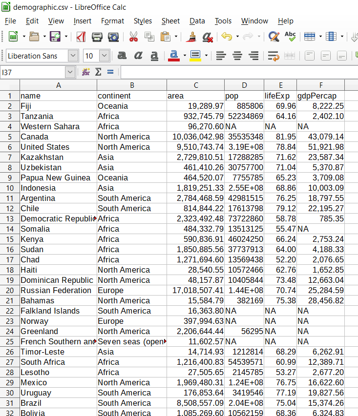
Figure 3.1: A screenshot of the sample dataset
We can import it with the read_csv() functions as:
demographic = read_csv("demographic.csv") Parsed with column specification:
cols(
name = col_character(),
continent = col_character(),
area = col_double(),
pop = col_double(),
lifeExp = col_double(),
gdpPercap = col_double()
)When read_csv() has imported the data into R workspace, it prints out the name and type of of data for each variable.
By simply glimpse the dataset, we see the format of the data is as expected. It has six variables(columns) and 177 observations (rows) similar to figure 3.1. Table 3.1 show sample of imported dataset. It contains six variables are name of the country, continent, areas of the country in square kilometer, population of the country, life expectancy and the GDP of the country in percent. The NA values indicates missing data in the data set.
| Country | Continent | Area (Km^2) | Population | Life Epectancy (Years) | GDP |
|---|---|---|---|---|---|
| Mauritania | Africa | 1054107.19 | 4063920 | 62.91 | 3655.39 |
| Bangladesh | Asia | 133782.14 | 159405279 | 71.80 | 2973.04 |
| Uzbekistan | Asia | 461410.26 | 30757700 | 71.04 | 5370.87 |
| Malawi | Africa | 111197.02 | 17068838 | 61.93 | 1090.37 |
| Vietnam | Asia | 335990.80 | 92544915 | 75.86 | 5264.83 |
| Brazil | South America | 8508557.09 | 204213133 | 75.04 | 15374.26 |
| Burundi | Africa | 26238.95 | 9891790 | 56.69 | 803.17 |
| Paraguay | South America | 401335.92 | 6552584 | 72.91 | 8501.54 |
| Trinidad and Tobago | North America | 7737.81 | 1354493 | 70.43 | 31181.82 |
| Timor-Leste | Asia | 14714.93 | 1212814 | 68.28 | 6262.91 |
| Palestine | Asia | 5037.10 | 4294682 | 73.13 | 4319.53 |
| Vanuatu | Oceania | 7490.04 | 258850 | 71.71 | 2892.34 |
3.2 Microsoft Excel(.xlsx)
Commonly our data is stored as a MS Excel file. we can import the file with read_xlsx() function of readxl package. The readxl package provides a function read_exel() that allows us to specify which sheet within the Excel file to read and what character specifies missing data (it assumes a blank cell is missing data if you don’t specifying anything). The function automatically convert the worksheet into a .csv file and read it.
audit = readxl::read_xlsx("audit.xlsx")The audit file is from the rattle package developed by Maindonald (2012). The dataset which is artificially constructed that has some of the charactersitcis of a true financial audit. I just saved it into the working directory as Excel spreadsheet. We will use this file to illustrate how to import the excel file into R workspace with readxl package (Wickham and Bryan 2018). We look on the internal structure of the audit file with the glimpse() function. You can interact with the table that show all variables and observations (Table 3.1)
audit%>%glimpse()## Observations: 2,000
## Variables: 13
## $ ID <dbl> 1004641, 1010229, 1024587, 1038288, 1044221, 1...
## $ Age <dbl> 38, 35, 32, 45, 60, 74, 43, 35, 25, 22, 48, 60...
## $ Employment <chr> "Private", "Private", "Private", "Private", "P...
## $ Education <chr> "College", "Associate", "HSgrad", "Bachelor", ...
## $ Marital <chr> "Unmarried", "Absent", "Divorced", "Married", ...
## $ Occupation <chr> "Service", "Transport", "Clerical", "Repair", ...
## $ Income <dbl> 81838.00, 72099.00, 154676.74, 27743.82, 7568....
## $ Gender <chr> "Female", "Male", "Male", "Male", "Male", "Mal...
## $ Deductions <dbl> 0, 0, 0, 0, 0, 0, 0, 0, 0, 0, 0, 0, 0, 0, 0, 0...
## $ Hours <dbl> 72, 30, 40, 55, 40, 30, 50, 40, 40, 37, 35, 40...
## $ IGNORE_Accounts <chr> "UnitedStates", "Jamaica", "UnitedStates", "Un...
## $ RISK_Adjustment <dbl> 0, 0, 0, 7298, 15024, 0, 22418, 0, 0, 0, 0, 0,...
## $ TARGET_Adjusted <dbl> 0, 0, 0, 1, 1, 0, 1, 0, 0, 0, 0, 0, 0, 0, 1, 0...DT::datatable(audit, rownames = FALSE, caption = "An Interactive table showing the audit data")Look the frequency
audit$Employment%>%table()## .
## Consultant NA Private PSFederal PSLocal PSState
## 148 100 1411 69 119 72
## SelfEmp Unemployed Volunteer
## 79 1 1audit$Gender%>%table()%>%barplot(horiz = TRUE)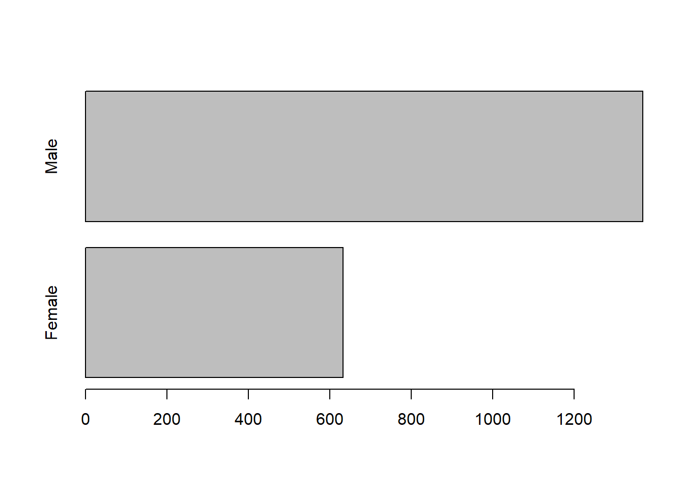
as.POSIXct("1920-10-12 10:05:3") %>% class()## [1] "POSIXct" "POSIXt"audit$Marital%>%table()%>%barplot(horiz = TRUE)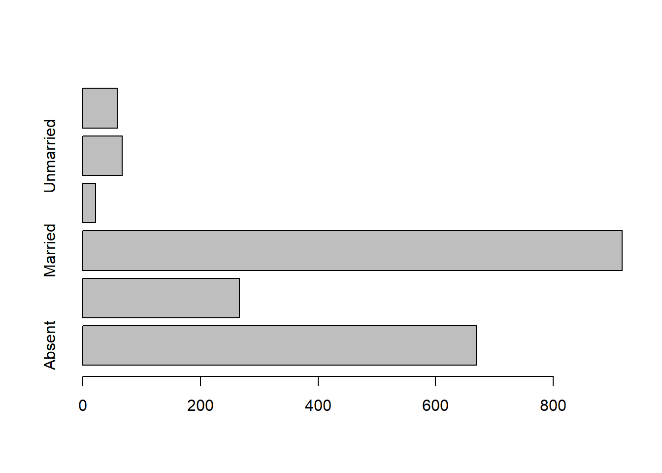
3.3 Writing t a File
Sometimes you work in the document and you want to export to a file. readr has write_csv() and write_tsv() functions that allows to export data frames from workspace to working directory
write_csv(audit, "audit.csv")
write_
Hadley and Grolemund (2016) recomment the use of write_excel_csv() function when you want to export a data frame to Excel. readr has other tools that export files to other software like SAS, SPSS and more …
write_excel_csv(audit, "audit.xls")3.4 Basic Data Manipulation
In this section, we brifely introduce some basic data handling and manipulation techniques, which are mostly associated with data frame. A data frame is a a tabular shaped contains columns and rows of equal length. In general a data frame structure with rows representing observations or measurements and with columns containing variables.
3.4.1 Explore the Data Frame
We can visualize the table by simply run the name of the data flights
flights = read_csv("flights.csv")## Warning: Missing column names filled in: 'X1' [1]## Parsed with column specification:
## cols(
## .default = col_integer(),
## carrier = col_character(),
## tailnum = col_character(),
## origin = col_character(),
## dest = col_character(),
## time_hour = col_character()
## )## See spec(...) for full column specifications.flights## # A tibble: 336,776 x 20
## X1 year month day dep_time sched_dep_time dep_delay arr_time
## <int> <int> <int> <int> <int> <int> <int> <int>
## 1 1 2013 1 1 517 515 2 830
## 2 2 2013 1 1 533 529 4 850
## 3 3 2013 1 1 542 540 2 923
## 4 4 2013 1 1 544 545 -1 1004
## 5 5 2013 1 1 554 600 -6 812
## 6 6 2013 1 1 554 558 -4 740
## 7 7 2013 1 1 555 600 -5 913
## 8 8 2013 1 1 557 600 -3 709
## 9 9 2013 1 1 557 600 -3 838
## 10 10 2013 1 1 558 600 -2 753
## # ... with 336,766 more rows, and 12 more variables: sched_arr_time <int>,
## # arr_delay <int>, carrier <chr>, flight <int>, tailnum <chr>,
## # origin <chr>, dest <chr>, air_time <int>, distance <int>, hour <int>,
## # minute <int>, time_hour <chr>we can use class() to check if the data is data frame
flights %>% class()## [1] "tbl_df" "tbl" "data.frame"We can use names() to extract the variable names
flights %>% names()## [1] "X1" "year" "month" "day"
## [5] "dep_time" "sched_dep_time" "dep_delay" "arr_time"
## [9] "sched_arr_time" "arr_delay" "carrier" "flight"
## [13] "tailnum" "origin" "dest" "air_time"
## [17] "distance" "hour" "minute" "time_hour"We can explore the internal structure of flights object with a dplyr()’s function glimpse()
flights %>% glimpse()## Observations: 336,776
## Variables: 20
## $ X1 <int> 1, 2, 3, 4, 5, 6, 7, 8, 9, 10, 11, 12, 13, 14, ...
## $ year <int> 2013, 2013, 2013, 2013, 2013, 2013, 2013, 2013,...
## $ month <int> 1, 1, 1, 1, 1, 1, 1, 1, 1, 1, 1, 1, 1, 1, 1, 1,...
## $ day <int> 1, 1, 1, 1, 1, 1, 1, 1, 1, 1, 1, 1, 1, 1, 1, 1,...
## $ dep_time <int> 517, 533, 542, 544, 554, 554, 555, 557, 557, 55...
## $ sched_dep_time <int> 515, 529, 540, 545, 600, 558, 600, 600, 600, 60...
## $ dep_delay <int> 2, 4, 2, -1, -6, -4, -5, -3, -3, -2, -2, -2, -2...
## $ arr_time <int> 830, 850, 923, 1004, 812, 740, 913, 709, 838, 7...
## $ sched_arr_time <int> 819, 830, 850, 1022, 837, 728, 854, 723, 846, 7...
## $ arr_delay <int> 11, 20, 33, -18, -25, 12, 19, -14, -8, 8, -2, -...
## $ carrier <chr> "UA", "UA", "AA", "B6", "DL", "UA", "B6", "EV",...
## $ flight <int> 1545, 1714, 1141, 725, 461, 1696, 507, 5708, 79...
## $ tailnum <chr> "N14228", "N24211", "N619AA", "N804JB", "N668DN...
## $ origin <chr> "EWR", "LGA", "JFK", "JFK", "LGA", "EWR", "EWR"...
## $ dest <chr> "IAH", "IAH", "MIA", "BQN", "ATL", "ORD", "FLL"...
## $ air_time <int> 227, 227, 160, 183, 116, 150, 158, 53, 140, 138...
## $ distance <int> 1400, 1416, 1089, 1576, 762, 719, 1065, 229, 94...
## $ hour <int> 5, 5, 5, 5, 6, 5, 6, 6, 6, 6, 6, 6, 6, 6, 6, 5,...
## $ minute <int> 15, 29, 40, 45, 0, 58, 0, 0, 0, 0, 0, 0, 0, 0, ...
## $ time_hour <chr> "1/1/2013 5:00", "1/1/2013 5:00", "1/1/2013 5:0...We can check how rows (observations/measurements) and columns (variables/fields) are in the data
flights %>% dim()## [1] 336776 20The number of rows (observation) can be obtained using nrow() function
flights %>% nrow()## [1] 336776The number of columns (variables) can be obtained using ncol() function
flights %>% ncol()## [1] 20The length of the data frame is given by
flights %>% length()## [1] 203.4.2 simmple summary statistics
The most helpful function for for summarizing rows and columns is summary(), which gives a collection of basim cummary statistics. The first method is to calculate some basic summary statistics (minimum, 25th, 50th, 75th percentiles, maximum and mean) of each column. If a column is categorical, the summary function will return the number of observations in each category.
flights %>% summary()## X1 year month day
## Min. : 1 Min. :2013 Min. : 1.000 Min. : 1.00
## 1st Qu.: 84195 1st Qu.:2013 1st Qu.: 4.000 1st Qu.: 8.00
## Median :168389 Median :2013 Median : 7.000 Median :16.00
## Mean :168389 Mean :2013 Mean : 6.549 Mean :15.71
## 3rd Qu.:252582 3rd Qu.:2013 3rd Qu.:10.000 3rd Qu.:23.00
## Max. :336776 Max. :2013 Max. :12.000 Max. :31.00
##
## dep_time sched_dep_time dep_delay arr_time
## Min. : 1 Min. : 106 Min. : -43.00 Min. : 1
## 1st Qu.: 907 1st Qu.: 906 1st Qu.: -5.00 1st Qu.:1104
## Median :1401 Median :1359 Median : -2.00 Median :1535
## Mean :1349 Mean :1344 Mean : 12.64 Mean :1502
## 3rd Qu.:1744 3rd Qu.:1729 3rd Qu.: 11.00 3rd Qu.:1940
## Max. :2400 Max. :2359 Max. :1301.00 Max. :2400
## NA's :8255 NA's :8255 NA's :8713
## sched_arr_time arr_delay carrier flight
## Min. : 1 Min. : -86.000 Length:336776 Min. : 1
## 1st Qu.:1124 1st Qu.: -17.000 Class :character 1st Qu.: 553
## Median :1556 Median : -5.000 Mode :character Median :1496
## Mean :1536 Mean : 6.895 Mean :1972
## 3rd Qu.:1945 3rd Qu.: 14.000 3rd Qu.:3465
## Max. :2359 Max. :1272.000 Max. :8500
## NA's :9430
## tailnum origin dest air_time
## Length:336776 Length:336776 Length:336776 Min. : 20.0
## Class :character Class :character Class :character 1st Qu.: 82.0
## Mode :character Mode :character Mode :character Median :129.0
## Mean :150.7
## 3rd Qu.:192.0
## Max. :695.0
## NA's :9430
## distance hour minute time_hour
## Min. : 17 Min. : 1.00 Min. : 0.00 Length:336776
## 1st Qu.: 502 1st Qu.: 9.00 1st Qu.: 8.00 Class :character
## Median : 872 Median :13.00 Median :29.00 Mode :character
## Mean :1040 Mean :13.18 Mean :26.23
## 3rd Qu.:1389 3rd Qu.:17.00 3rd Qu.:44.00
## Max. :4983 Max. :23.00 Max. :59.00
## You noticed that the summary() function provide the common metric for central tendency and measure of dispersion. We will look at them later. Now we turn to our favourite package dplyr
References
Matthew, Crump. 2018. Programming for Psychologists: Data Creation and Analysis. Book. Mathhew Crump.
Maindonald, John H. 2012. “Data Mining with Rattle and R: The Art of Excavating Data for Knowledge Discovery by Graham Williams.” International Statistical Review 80 (1). Wiley Online Library: 199–200.
Wickham, Hadley, and Jennifer Bryan. 2018. Readxl: Read Excel Files. https://CRAN.R-project.org/package=readxl.
Hadley, Wickham, and Garrett Grolemund. 2016. R for Data Science. Book. O’Reilly Media.