Chapter 5 Reshaping data with tidyr
It is often said that 80% of data analysis is spent on the cleaning and preparing data (Hadley and Grolemund 2016). And it’s not just a first step, but it must be repeated many times over the course of analysis as new problems come to light or new data is collected. Most of the time, our data is in the form of a data frame and we are interested in exploring the relationships(R Core Team 2018). However most procedures in R expect the data to show up in a ‘long’ format where each row is an observation and each column is a variable (Wickham and Henry 2018; Wickham et al. 2018). In practice, the data is often not stored like that and the data comes to us with repeated observations included on a single row. This is often done as a memory saving technique or because there is some structure in the data that makes the ‘wide’ format attractive. As a result, we need a way to convert data from wide5 to long6 and vice-versa (Matthew 2018).
Data structure can become an issue when using statistical software packages, as some program prefer long format while others prefer wide format. For example, repeated-measures ANOVAs works with wide format, but between-subjects ANOVAs works well in long-format and mixed design ANOVAs work with both. dplyr, ggplot2, and all the other packages in the tidyverse for example work with long format data structure (Wickham 2017). In R, many of the statistics packages require the data to be in long-format (R Core Team 2018). It is important to become comfortable with either format, and with techniques for transforming data between formats. Therefore, the principles of tidy data provide a standard way to organise data values within a dataset either in long or wide format. And tidyr package was built for the sole purpose of simplifying the process of tranforming these two types of data structures depending on the requirement (Wickham and Henry 2018). This chapeter provides you with the basic understanding of the four fundamental functions of data tidying the data and structure it to format that make data analysis easy. These function include:
gather()makes “wide” data longerspread()makes “long” data widerseparate()splits a single column into multiple columnsunite()combines multiple columns into a single column
require(dplyr)
require(readr)
require(lubridate)
require(readxl)
require(haven)
require(ggplot2)
require(kableExtra)
require(tidyr)
5.1 gather( ) function:
There are times when our data is considered unstacked and a common attribute of concern is spread out across columns. To reformat the data such that these common attributes are gathered together as a single variable, the gather() function will take multiple columns and collapse them into key-value pairs, duplicating all other columns as needed. in short gather() function reshape wide format to long format (Figure 5.1)
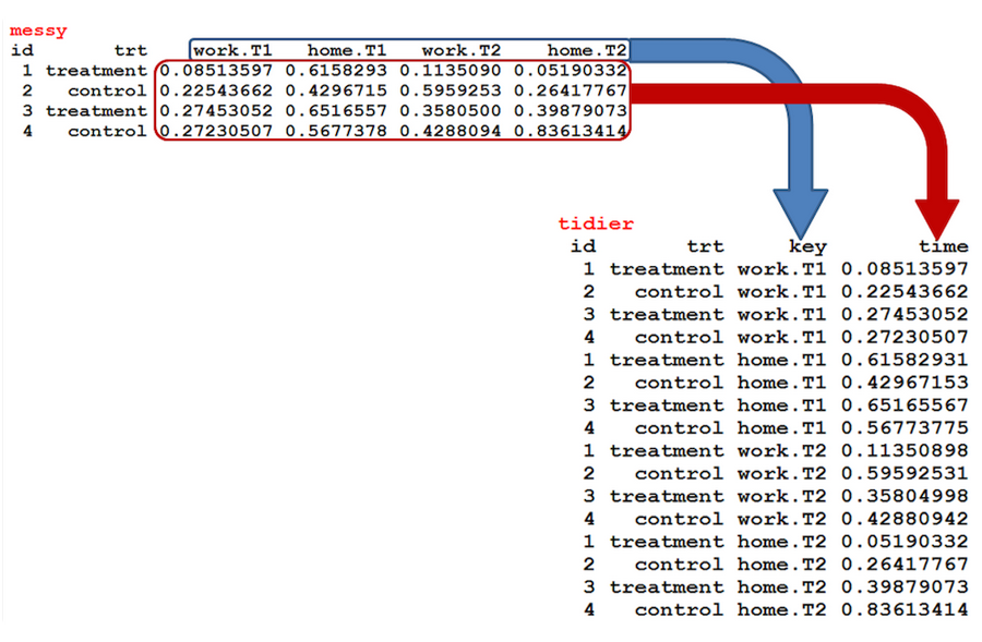
Figure 5.1: Reshaped data set from wide to long format
The data in table 5.1 data is considered wide since the time variable (represented as quarters) is structured such that each quarter represents a variable. To re-structure the time component as an individual variable, we can gather each quarter within one column variable and also gather the values associated with each quarter in a second column variable.
wide = read_table2("wide_data.txt")## Parsed with column specification:
## cols(
## Group = col_integer(),
## Year = col_integer(),
## Qtr.1 = col_integer(),
## Qtr.2 = col_integer(),
## Qtr.3 = col_integer(),
## Qtr.4 = col_integer()
## )wide %>%
kable("html", caption = "Revenue data in Wide form")%>%
column_spec(column = 1:6, width = "3cm", color = 1) %>%
add_header_above(c("" , "", "Income per Quarter" = 4), line = T)| Group | Year | Qtr.1 | Qtr.2 | Qtr.3 | Qtr.4 |
|---|---|---|---|---|---|
| 1 | 2006 | 15 | 16 | 19 | 17 |
| 1 | 2007 | 12 | 13 | 27 | 23 |
| 1 | 2008 | 22 | 22 | 24 | 20 |
| 1 | 2009 | 10 | 14 | 20 | 16 |
| 2 | 2006 | 12 | 13 | 25 | 18 |
| 2 | 2007 | 16 | 14 | 21 | 19 |
| 2 | 2008 | 13 | 11 | 29 | 15 |
| 2 | 2009 | 23 | 20 | 26 | 20 |
| 3 | 2006 | 11 | 12 | 22 | 16 |
| 3 | 2007 | 13 | 11 | 27 | 21 |
| 3 | 2008 | 17 | 12 | 23 | 19 |
| 3 | 2009 | 14 | 9 | 31 | 24 |
We use the gather() function to convert data in table 5.1 to long form widely known as indexed data shown in table 5.2
long = wide %>%
gather(key = "key", value = "Revenue", 3:6)| Group | Year | key | Revenue |
|---|---|---|---|
| 1 | 2006 | Qtr.1 | 15 |
| 1 | 2007 | Qtr.1 | 12 |
| 1 | 2008 | Qtr.1 | 22 |
| 1 | 2009 | Qtr.1 | 10 |
| 2 | 2006 | Qtr.1 | 12 |
| 2 | 2007 | Qtr.1 | 16 |
| 2 | 2008 | Qtr.1 | 13 |
| 2 | 2009 | Qtr.1 | 23 |
| 3 | 2006 | Qtr.1 | 11 |
| 3 | 2007 | Qtr.1 | 13 |
| 3 | 2008 | Qtr.1 | 17 |
| 3 | 2009 | Qtr.1 | 14 |
| 1 | 2006 | Qtr.2 | 16 |
| 1 | 2007 | Qtr.2 | 13 |
| 1 | 2008 | Qtr.2 | 22 |
| 1 | 2009 | Qtr.2 | 14 |
| 2 | 2006 | Qtr.2 | 13 |
| 2 | 2007 | Qtr.2 | 14 |
| 2 | 2008 | Qtr.2 | 11 |
| 2 | 2009 | Qtr.2 | 20 |
| 3 | 2006 | Qtr.2 | 12 |
| 3 | 2007 | Qtr.2 | 11 |
| 3 | 2008 | Qtr.2 | 12 |
| 3 | 2009 | Qtr.2 | 9 |
| 1 | 2006 | Qtr.3 | 19 |
| 1 | 2007 | Qtr.3 | 27 |
| 1 | 2008 | Qtr.3 | 24 |
| 1 | 2009 | Qtr.3 | 20 |
| 2 | 2006 | Qtr.3 | 25 |
| 2 | 2007 | Qtr.3 | 21 |
| 2 | 2008 | Qtr.3 | 29 |
| 2 | 2009 | Qtr.3 | 26 |
| 3 | 2006 | Qtr.3 | 22 |
| 3 | 2007 | Qtr.3 | 27 |
| 3 | 2008 | Qtr.3 | 23 |
| 3 | 2009 | Qtr.3 | 31 |
| 1 | 2006 | Qtr.4 | 17 |
| 1 | 2007 | Qtr.4 | 23 |
| 1 | 2008 | Qtr.4 | 20 |
| 1 | 2009 | Qtr.4 | 16 |
| 2 | 2006 | Qtr.4 | 18 |
| 2 | 2007 | Qtr.4 | 19 |
| 2 | 2008 | Qtr.4 | 15 |
| 2 | 2009 | Qtr.4 | 20 |
| 3 | 2006 | Qtr.4 | 16 |
| 3 | 2007 | Qtr.4 | 21 |
| 3 | 2008 | Qtr.4 | 19 |
| 3 | 2009 | Qtr.4 | 24 |
The spread() function is a complement functiongather()` as it convert long format dataset into wide form
wide.wide = long %>% spread(key = "key", value = "Revenue")5.2 separate( ) function:
Many times a single column variable will capture multiple variables, or even parts of a variable you just don’t care about. Examples include is data in table 5.3).
usa = read_csv("separate.csv")## Parsed with column specification:
## cols(
## Grp_Ind = col_character(),
## Yr_Mo = col_character(),
## City_State = col_character(),
## First_Last = col_character(),
## Extra_variable = col_character()
## )| Grp_Ind | Yr_Mo | City_State | First_Last | Extra_variable |
|---|---|---|---|---|
| 1.a | 2006_Jan | Dayton (OH) | George Washington | XX01person_1 |
| 1.b | 2006_Feb | Grand Forks (ND) | John Adams | XX02person_2 |
| 1.c | 2006_Mar | Fargo (ND) | Thomas Jefferson | XX03person_3 |
| 2.a | 2007_Jan | Rochester (MN) | James Madison | XX04person_4 |
| 2.b | 2007_Feb | Dubuque (IA) | James Monroe | XX05person_5 |
| 2.c | 2007_Mar | Ft. Collins (CO) | John Adams | XX06person_6 |
| 3.a | 2008_Jan | Lake City (MN) | Andrew Jackson | XX07person_7 |
| 3.b | 2008_Feb | Rushford (MN) | Martin Van Buren | XX08person_8 |
| 3.c | 2008_Mar | Unknown | William Harrison | XX09person_9 |
In each of these cases, our objective may be to separate characters within the variable string. This can be accomplished using the separate() function which splits a single variable into multiple variables. Table 5.4 show the tidy data after the variables were separated. The complement function to separate() is the unite(), which merge two variables into one.
usa.sep = usa %>%
  separate(Grp_Ind, c("Group", "Individual"),  remove = TRUE, convert = TRUE) %>%
  separate(Yr_Mo, c("Year", "Month"),  remove = TRUE, convert = TRUE) %>%
  separate(City_State, c("City", "State"),  remove = TRUE, convert = TRUE) %>%
  separate(First_Last, c("First", "Last"),  remove = TRUE, convert = TRUE) %>%
  separate(Extra_variable, c("Extra", "Variable"),  remove = TRUE, convert = TRUE)
## Warning: Expected 2 pieces. Additional pieces discarded in 8 rows [1, 2, 3,
## 4, 5, 6, 7, 8].## Warning: Expected 2 pieces. Missing pieces filled with `NA` in 1 rows [9].## Warning: Expected 2 pieces. Additional pieces discarded in 1 rows [8].| Group | Individual | Year | Month | City | State | First | Last | Extra | Variable |
|---|---|---|---|---|---|---|---|---|---|
| 1 | a | 2006 | Jan | Dayton | OH | George | Washington | XX01person | 1 |
| 1 | b | 2006 | Feb | Grand | Forks | John | Adams | XX02person | 2 |
| 1 | c | 2006 | Mar | Fargo | ND | Thomas | Jefferson | XX03person | 3 |
| 2 | a | 2007 | Jan | Rochester | MN | James | Madison | XX04person | 4 |
| 2 | b | 2007 | Feb | Dubuque | IA | James | Monroe | XX05person | 5 |
| 2 | c | 2007 | Mar | Ft | Collins | John | Adams | XX06person | 6 |
| 3 | a | 2008 | Jan | Lake | City | Andrew | Jackson | XX07person | 7 |
| 3 | b | 2008 | Feb | Rushford | MN | Martin | Van | XX08person | 8 |
| 3 | c | 2008 | Mar | Unknown | NA | William | Harrison | XX09person | 9 |
References
Hadley, Wickham, and Garrett Grolemund. 2016. R for Data Science. Book. O’Reilly Media.
R Core Team. 2018. R: A Language and Environment for Statistical Computing. Vienna, Austria: R Foundation for Statistical Computing. https://www.R-project.org/.
Wickham, Hadley, and Lionel Henry. 2018. Tidyr: Easily Tidy Data with ’Spread()’ and ’Gather()’ Functions. https://CRAN.R-project.org/package=tidyr.
Wickham, Hadley, Romain François, Lionel Henry, and Kirill Müller. 2018. Dplyr: A Grammar of Data Manipulation. https://CRAN.R-project.org/package=dplyr.
Matthew, Crump. 2018. Programming for Psychologists: Data Creation and Analysis. Book. Mathhew Crump.
Wickham, Hadley. 2017. Tidyverse: Easily Install and Load the ’Tidyverse’. https://CRAN.R-project.org/package=tidyverse.