Machine learning with tidymodels: Linear and Bayesian Regression Models

Introduction
We live in age of increasing data and as a data scientist, our role primarily involves exploring and analyzing data. However, with the amount of data data exploration and analysis become a thing for automation and use of intelligent tools to help us glean key information from data. The results of an analysis might form the basis of a report or a machine learning model, but it all begins with data. The two popular tools commonly used are R and Python. R is one of the most popular programming languages for data scientists. R is an elegant environment that’s designed to support data science, and you can use it for many purposes.
After decades of open-source development, R provides extensive functionality that’s backed by a massive set of powerful statistical modeling, machine learning, visualization and data wrangling packages. Some of these package that has revolutionized R are tidyverse and tidymodel package. tidyverse is a collection of R packages that make data science faster, easier, and more fun and tidymodels is a collection of R packages for modeling and statistical analysis.
As a data scientist, you need to distinguish between regression predictive models and classification predictive models. Clear understanding of these models helps to choose the best one for a specific use case. In a nutshell, regression predictive modelsand classification predictive models fall under supervised machine learning. The main difference between these two models is the output: while in regression produce an output as numerical (or continuous), the output of classification is categorical (or discrete).
A big part of machine learning is classification — we want to know what class or group an observation belongs to. Therefore, the ability to precisely classify observations to their groups is valuable for various business applications like predicting the future based on historical data. For example, when provided with a dataset about environmental variables, and you are asked to predict productivity, that is a regression task because productivity measured in term of chlorophyll concentration will be a continuous output.
In this post we will focus on regression. We will learn the steps of modelling using tidymodels (Kuhn and Wickham, 2020a). We first explore the data and check if it fit for modelling, we then split the dataset into a training and testing sets. Next, we will create a recipe object and define our model. Lastly, we will train a specified model and evaluate its performance. I will use the same dataset for three different model’s algorithms. Example of the common regression algorithms include random forest, linear regression, support vector regression (SVR) and bayes. Some algorithms, such as logistic regression, have the name regression in their functions but they are not regression algorithms.
To follow use code in this article, you will need tidymodels (Kuhn and Wickham, 2020a) and tidyverse packages (Wickham and Wickham, 2017) installed in your machine. You can install them from CRAN. The chunk below highlight lines of code to install the packages if they are yet in your PC.
similar to the tidyverse, tidymodels consists of several linked packages that use a similar philosophy and syntax. Here is a brief explanation of the component packages.
- parsnips: used to define models using a common syntax; makes it easier to experiment with different algorithms
- workflows: provides tools to create workflows, or the desired machine learning pipeline, including pre-processing, training, and post-processing
- yardstick: a one-stop-shop to implement a variety of assessment metrics for regression and classification problems
- tune: for hyperparameter tuning
- dials: for managing parameters and tuning grids
- rsample: tools for data splitting, partitioning, and resampling
- recipes: tools for pre-processing and data engineering
Once installed, you can load the packages in your session. I begin by reading in the required packages. Here, tidymodels is used to load the component packages discussed above along with some other packages (e.g., ggplot2, purr, and dplyr).
The dataset
We use the data collected with the Institute of Marine Sciences of the University of Dar es Salaam to illustrate the concept. The data was collected through the Coral Reef Targeted Research and Capacity Building for Management (CRTR) project between 2008 and 2009. The dataset contains;
- Chemical variables —nitrate, phosphate, salinity, pH, dissolved oxygen and ammonia
- Physical variables — temperature
- Biological variables— chlorophyll-a
Because the variables are organized in sheets of Excel spreadsheet, i used a read_excel function from readxl package (Wickham and Bryan, 2018) to read the file from the sheet. And because there are several sheet, the processed was iterated with a for loop. Data from each sheet was allocated in the list file. The chunk below highlight the code used to read files in sheets.
The data was untidy and unsuitable for visualization and modelling in R. Therefore, the first thing I had to deal with the data was to tidy the variables in the dataset to a right format that tidymodels and tidyverse recognizes. First the dataset was unlisted with bind_rows function and the data was pivoted to long format and then back to wide format with only the variable of interested selected.
## organize in long form
crtr.long = crtr.list %>%
  bind_rows() %>%
  pivot_longer(cols =2:5, names_to = "sites", values_to = "data" )

## organize in the wide form
crtr.wide = crtr.long %>%
  pivot_wider(names_from = variable, values_from = data) %>%
  mutate(month = lubridate::month(Date, label = TRUE,
                                  abb = TRUE) %>% as.character()) %>%
  mutate_if(is.character, as.factor) %>%
  mutate_if(is.numeric, round, digits = 2)  %>%
  select(date = Date, month,sites, chl, everything())
Let’s us glimpse the dataset
Rows: 52
Columns: 11
$ date        <dttm> 2008-03-01, 2008-03-01, 2008-03-01, 2008-03-01, 2008-04-0~
$ month       <fct> Mar, Mar, Mar, Mar, Apr, Apr, Apr, Apr, May, May, May, May~
$ sites       <fct> Pongwe, Mnemba, Chumbe, Bawe, Pongwe, Mnemba, Chumbe, Bawe~
$ chl         <dbl> 0.09, 0.26, 0.56, 0.43, 0.47, 1.01, 0.63, 1.39, 0.37, 0.33~
$ salinity    <dbl> 35.0, 34.0, 32.0, 32.0, 35.0, 35.0, 34.0, 34.0, 36.0, 36.0~
$ temperature <dbl> 28.8, 28.4, 28.0, 28.0, 28.2, 27.7, 28.1, 26.7, 27.0, 27.2~
$ do          <dbl> 6.11, 5.95, 6.16, NA, 6.35, 6.14, 7.01, 6.31, 6.15, 6.10, ~
$ ph          <dbl> 7.86, 7.88, 7.73, NA, 7.87, 7.88, 7.86, 7.91, 7.68, 7.80, ~
$ ammonia     <dbl> 0.55, 0.80, 0.74, 0.94, 0.56, 0.72, 0.53, 0.97, 0.56, 0.65~
$ phosphate   <dbl> 0.28, 0.28, 1.31, 1.91, 0.28, 0.32, 1.16, 0.84, 0.28, 0.43~
$ nitrate     <dbl> 0.04, 0.07, 3.26, 3.34, 0.03, 0.47, 1.45, 0.84, 0.06, 0.48~
As a first step in modeling, it’s always a good idea to explore the variables in the dataset. Figure 1 is a pairplot that compare each pair of variables as scatterplots in the lower diagonal, densities on the diagonal and correlations written in the upper diagonal (Schloerke et al., 2020). Figure 2 show the correlation between chlorophyll-a (outcome) with other six predictor variables using a linear and quadratic equations is unfit for these dataset.
crtr.wide %>%
  select(-salinity)%>%
  mutate(season = lubridate::month(date) %>% as.integer(),
         season = replace(season,season %in% c(1:4,11:12), "NE"),
         season = replace(season,season %in% c(5:10), "SE"))%>%
  GGally::ggscatmat(columns = 4:10,color="season", alpha=1, corMethod = "spearman")+
  ggsci::scale_color_jco()+
  ggpubr::theme_pubclean()+
  theme(strip.background = element_blank(),
        legend.position = "right",
        legend.key = element_blank())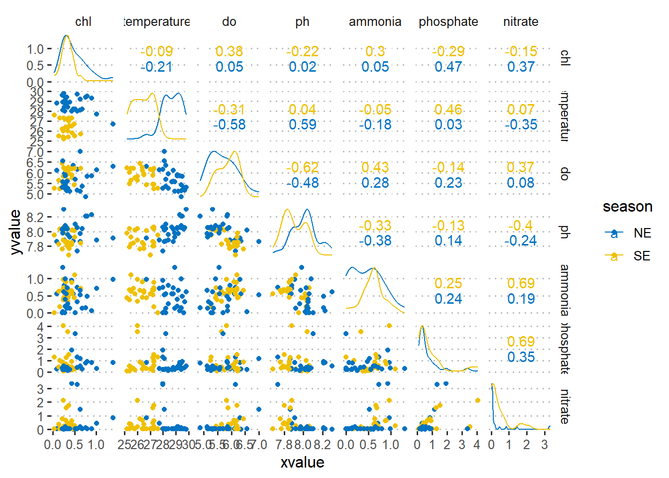
wesa = wesanderson::wes_palettes %>% names()

crtr.wide %>%
  select(-salinity)%>%
  filter(nitrate < 1 & phosphate < 1.2 & chl < 1) %>%
  pivot_longer(cols = 5:10, names_to = "predictor", values_to = "data") %>%
  # filter(sites == "Bawe")%>%
  ggplot(aes(x = data, y = chl))+
  scale_y_continuous(trans = scales::sqrt_trans(), labels = function(x) round(x,2))+
  # scale_x_continuous(trans = scales::sqrt_trans(), labels = function(x) round(x,2))+
  geom_jitter()+
  geom_smooth(se = FALSE, method = "lm", formula = "y ~ poly(x,2)", aes(color = "Quadratic"))+
  geom_smooth(se = FALSE, method = "lm", formula = "y ~ x", aes(color = "Linear"))+
   ggsci::scale_color_jco()+
  facet_wrap(~predictor, scales = "free_x")+
  ggpubr::theme_pubclean()+
  theme(strip.background.x = element_blank(), legend.key = element_blank(),
        legend.position = "right", panel.background = element_rect(colour = "black"))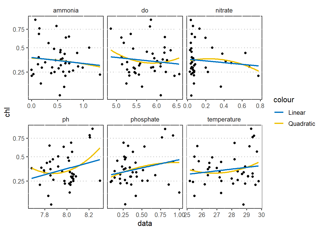
Resample
In machine learning, one risk is the machine learns too well our sample data and is then less accurate during a real-world testing. This phenomenon is called overtraining or overfitting. We overcome this problem by splitting the dataset into a training and testing sets. The training set is used to train the model while the test set is reserved to later estimate how well the model might work on new or wild data. The splitting is based on ratios and the widely used ratios include 80/20, 75/25, or 7/30, with the training data receiving a bigger proportion of the dataset and the test set get the remaining small portion.
For our sample that has only 52 observations, it make sense to use 70/30 split ratio. we use the fraction set.seed(4595) from base R to fix the random number generator from rsample package (Kuhn et al., 2020). This prevent generating new data in each execution. the function initial_split from the rsample package is designed to split the dataset into a training and testing sets. We purse the data to be split and the proportion that serve as a cutpoint of the two sets.
<Analysis/Assess/Total>
<28/13/41>
Given the 41 total observations, we reserve 12 observations as a test set and kept 70% of the dataset (29 observation) as train set. From the crtr.split object, we pull both the train set with the training function and the test set with a testing function.
We can have a glimpse of the train dataset using a glimpse function from dplyr package (Wickham et al., 2019).
Rows: 28
Columns: 7
$ chl         <dbl> 0.44, 0.37, 0.25, 0.23, 0.47, 0.68, 0.45, 0.28, 0.33, 0.63~
$ temperature <dbl> 27.3, 27.0, 29.8, 28.9, 28.2, 28.2, 25.8, 27.2, 27.2, 29.2~
$ do          <dbl> 6.19, 6.15, 5.32, 5.56, 6.35, 5.36, 5.76, 5.46, 6.10, 5.12~
$ ph          <dbl> 7.85, 7.68, 8.30, 7.98, 7.87, 8.04, 8.02, 8.05, 7.80, 7.97~
$ ammonia     <dbl> 0.88, 0.56, 0.61, 1.32, 0.56, 0.14, 0.56, 0.52, 0.65, 0.66~
$ phosphate   <dbl> 0.92, 0.28, 0.51, 0.30, 0.28, 0.26, 0.17, 0.14, 0.43, 0.54~
$ nitrate     <dbl> 0.64, 0.06, 0.03, 0.04, 0.03, 0.05, 0.05, 0.04, 0.48, 0.20~
The printed output shows that we have seven variables and all are numeric
recipe
The recipes package (Kuhn and Wickham, 2020b) define a recipe object that we will use for modeling and to conduct preprocessing of variables. The four main functions are recipe(), prep(), juice() and bake(). recipe() defines the operations on the data and the associated roles. Once the preprocessing steps are defined, any parameters are estimated using prep().
Recipes can be created manually by sequentially adding roles to variables in a data set. First, we will create a recipe object from the train set data and then specify the processing steps and transform the data with step_*. once the recipe is ready we prep it. For example, to create a simple recipe containing only an outcome and predictors and have the predictors normalized and missing values in predictors imputed:
crtr.recipe = crtr.train %>%
  recipe(chl ~ .) %>%
  step_normalize(all_numeric()) %>%
  step_corr(all_numeric())%>%
  step_impute_knn(all_numeric()) %>%
  prep()

crtr.recipe
Recipe
Inputs:
role #variables
outcome 1
predictor 6
Training data contained 28 data points and no missing data.
Operations:
Centering and scaling for temperature, do, ph, ammonia, phosphate, nitrat... [trained]
Correlation filter on <none> [trained]
K-nearest neighbor imputation for temperature, do, ph, ammonia, phosphate, nitra... [trained]Once the data are ready for transformation, the juices() extract transformed training set while the bake() function create a new testing set.
Build Models
Random Forest
We begin by fitting a random forest model.
Make random forest model
We specify the model using the parsnip package (Kuhn and Vaughan, 2020a). This package provides a tidy, unified interface to models for a range of models without getting bogged down in the syntactical minutiae of the underlying packages. The parsnip package help us to specify ;
- the
typeof model e.g random forest, - the
modeof the model whether isregressionorclassification - the computational
engineis the name of the R package.
Based on the information above, we can use parsnip package to build our model as;
Train random forest model
Once we have specified the model type, engine and mode, the model can be trained with the fit function. We simply parse into the fit the specified model and the transformed training set extracted from the prepped recipe.
predict with random forest
To get our predicted results, we use the predict() function to find the estimated chlorophyll-a. First, let’s generate the estimated chlorophyll-a values by simply parse the random forest model rf.model we specified and the transformed testing set we created from a prepped recipe. We also stitch the predicted values to the transformed train set with bind_cols function;
# A tibble: 13 x 8
     .pred temperature      do     ph ammonia phosphate nitrate     chl
     <dbl>       <dbl>   <dbl>  <dbl>   <dbl>     <dbl>   <dbl>   <dbl>
 1 -0.143        0.407  0.624  -0.756  1.05     -0.485   -0.364 -0.685
 2 -0.0964      -0.897  0.603  -1.56   0.401    -0.242   -0.419 -0.0561
 3 -0.0919      -0.897  0.516  -1.20   0.530     0.0808   1.32   0.206
 4  0.366       -1.10   1.69   -1.64   0.562     1.86     3.49  -0.894
 5 -0.0544      -0.966  1.30   -0.976 -0.0507   -0.565   -0.364 -0.161
 6 -0.0748      -1.58  -0.0480 -1.12   0.498     0.0808   1.26  -1.31
 7  0.0753      -1.58   1.17   -0.462  2.05     -0.525    0.721  0.573
 8  0.160        0.887  0.538   0.493 -0.244     0.121   -0.473 -0.528
 9  0.189        0.887  0.429   0.420 -0.890    -0.202    0.341 -0.528
10 -0.0890       0.132 -0.850   0.567 -1.54     -0.767   -0.419 -0.632
11 -0.386        0.613 -0.200   0.567  0.272    -0.767   -0.364 -0.423
12 -0.0471       1.09  -0.503   0.714  1.66     -0.162   -0.419 -0.528
13  0.800        1.16   0.386   1.67   0.0138    2.10    -0.419  2.09
When making predictions, the tidymodels convention is to always produce a tibble of results with standardized column names. This makes it easy to combine the original data and the predictions in a usable format:
Evaluate the rf model
So far, we have built a model and preprocessed data with a recipe. We predicted new data as a way to bundle a parsnip model and recipe together. The next step is to assess or evaluate the accuracy of the model. We use a metrics function from yardstick package (Kuhn and Vaughan, 2020b)to assess the accuracy of the model by comparing the predicted versus the original outcome variable. Note that we use the predicted dataset we just computed using predict function.
Linear regression approach
Make linear model
The good of tidymodels is that when we change the model, we do not need to start over again from the beginning but rather change the engine. For instance, we replace the ranger engine with lm to specify the linear model using the parsnip package (Kuhn and Vaughan, 2020a) .
Train Linear model
Once we have specified the model type, engine and mode, the model can be trained with the fit function;
Predict with linear model
Once the model is fitted, This fitted object lm_fit has the lm model output built-in, which you can access with lm_fit$fit, but there are some benefits to using the fitted parsnip model object when it comes to predicting. To predict the values we use predict function and parse the model and standardized testing values we computed from the recipe (R Core Team, 2018). Note that here we use the transformed test set and not the original from the split object. In this case we use the model to predict the value and stitch the testing values using the bind_cols function;
# A tibble: 13 x 8
     .pred temperature      do     ph ammonia phosphate nitrate     chl
     <dbl>       <dbl>   <dbl>  <dbl>   <dbl>     <dbl>   <dbl>   <dbl>
 1 -0.347        0.407  0.624  -0.756  1.05     -0.485   -0.364 -0.685
 2 -0.239       -0.897  0.603  -1.56   0.401    -0.242   -0.419 -0.0561
 3 -0.260       -0.897  0.516  -1.20   0.530     0.0808   1.32   0.206
 4  0.0430      -1.10   1.69   -1.64   0.562     1.86     3.49  -0.894
 5 -0.238       -0.966  1.30   -0.976 -0.0507   -0.565   -0.364 -0.161
 6 -0.243       -1.58  -0.0480 -1.12   0.498     0.0808   1.26  -1.31
 7 -0.614       -1.58   1.17   -0.462  2.05     -0.525    0.721  0.573
 8  0.142        0.887  0.538   0.493 -0.244     0.121   -0.473 -0.528
 9  0.0942       0.887  0.429   0.420 -0.890    -0.202    0.341 -0.528
10  0.115        0.132 -0.850   0.567 -1.54     -0.767   -0.419 -0.632
11 -0.191        0.613 -0.200   0.567  0.272    -0.767   -0.364 -0.423
12 -0.215        1.09  -0.503   0.714  1.66     -0.162   -0.419 -0.528
13  0.760        1.16   0.386   1.67   0.0138    2.10    -0.419  2.09
Evaluate linear model
Once we have our lm.predict dataset that contains the predicted and test values, we can now use the metrics fiction to evaluate the accuracy of the model.
Estimate stats
Sometimes you may wish to plot predicted values with different predictors. To do that you need to create a new tidied data from the the model with tidy function and parse interval = TRUE argument as shown in the code below. This create a tibble shown below and the same data is plotted in figure @ref(fig:fig3).
# A tibble: 7 x 5
  term         estimate std.error statistic p.value
  <chr>           <dbl>     <dbl>     <dbl>   <dbl>
1 (Intercept) -3.41e-17     0.200 -1.71e-16   1
2 temperature  1.29e- 2     0.253  5.09e- 2   0.960
3 do          -2.09e- 2     0.261 -8.00e- 2   0.937
4 ph           6.88e- 2     0.289  2.38e- 1   0.814
5 ammonia     -1.63e- 1     0.235 -6.96e- 1   0.494
6 phosphate    2.91e- 1     0.277  1.05e+ 0   0.306
7 nitrate     -6.99e- 2     0.316 -2.21e- 1   0.827
lm.fit.stats %>%
slice(-1) %>%
ggplot(aes(x = term, y = estimate)) +
geom_point(size = 4)+
geom_errorbar(aes(ymin = estimate-std.error, ymax = estimate+std.error), width = .2)+
scale_y_continuous(breaks = seq(-1.5,1.5,0.5))+
ggpubr::theme_pubclean()+
theme(axis.text = element_text(size = 10))+
labs(x = "", y = "Estimated chl")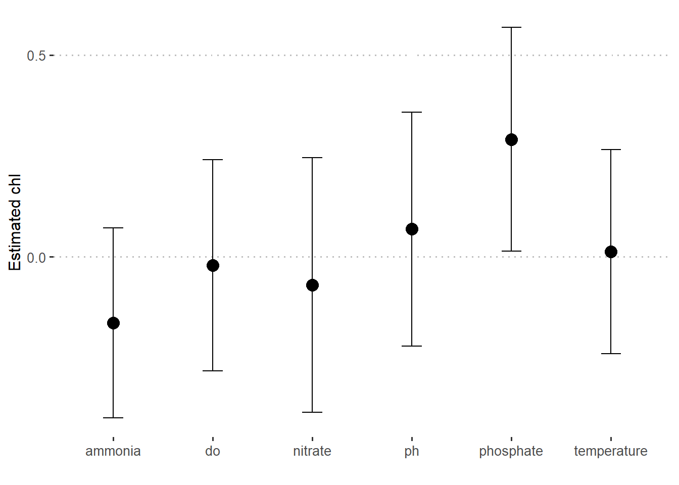
Bayesian approach
Make Bayes Model
For Bayesian, we also change the engine and specified are called prior and prior_intercept. It turns out that linear_reg() has a stan engine. Since these prior distribution arguments are specific to the Stan software, they are passed as arguments to parsnip::set_engine().
This kind of Bayesian analysis (like many models) involves randomly generated numbers in its fitting procedure. We can use set.seed() to ensure that the same (pseudo-)random numbers are generated each time we run this code. The number 123 isn’t special or related to our data; it is just a “seed” used to choose random numbers.
Train Bayes model
Once we have defined the Bayesian model, we train it using a transformed testing set;
parsnip model object

stan_glm
 family:       gaussian [identity]
 formula:      chl ~ .
 observations: 13
 predictors:   7
------
            Median MAD_SD
(Intercept) -0.2    0.2
temperature -0.5    0.3
do           0.4    0.4
ph           0.6    0.4
ammonia      0.1    0.2
phosphate    0.6    0.3
nitrate     -0.5    0.3

Auxiliary parameter(s):
      Median MAD_SD
sigma 0.7    0.2

------
* For help interpreting the printed output see ?print.stanreg
* For info on the priors used see ?prior_summary.stanreg
Predict Bayes fit
# A tibble: 13 x 8
     .pred temperature      do     ph ammonia phosphate nitrate     chl
     <dbl>       <dbl>   <dbl>  <dbl>   <dbl>     <dbl>   <dbl>   <dbl>
 1 -0.607        0.407  0.624  -0.756  1.05     -0.485   -0.364 -0.685
 2 -0.302       -0.897  0.603  -1.56   0.401    -0.242   -0.419 -0.0561
 3 -0.827       -0.897  0.516  -1.20   0.530     0.0808   1.32   0.206
 4 -0.617       -1.10   1.69   -1.64   0.562     1.86     3.49  -0.894
 5  0.0850      -0.966  1.30   -0.976 -0.0507   -0.565   -0.364 -0.161
 6 -0.611       -1.58  -0.0480 -1.12   0.498     0.0808   1.26  -1.31
 7  0.379       -1.58   1.17   -0.462  2.05     -0.525    0.721  0.573
 8  0.0950       0.887  0.538   0.493 -0.244     0.121   -0.473 -0.528
 9 -0.686        0.887  0.429   0.420 -0.890    -0.202    0.341 -0.528
10 -0.705        0.132 -0.850   0.567 -1.54     -0.767   -0.419 -0.632
11 -0.516        0.613 -0.200   0.567  0.272    -0.767   -0.364 -0.423
12 -0.256        1.09  -0.503   0.714  1.66     -0.162   -0.419 -0.528
13  1.74         1.16   0.386   1.67   0.0138    2.10    -0.419  2.09
Evaluate Bayes model
Bayes.fit.stats
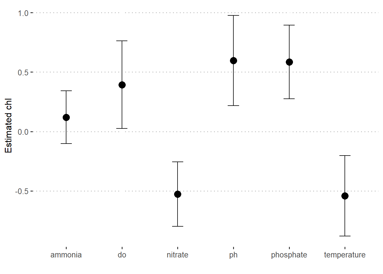
To update the parameter table, the tidy() method is once again used:
# A tibble: 7 x 3
  term        estimate std.error
  <chr>          <dbl>     <dbl>
1 (Intercept)   -0.220     0.230
2 temperature   -0.541     0.338
3 do             0.394     0.370
4 ph             0.597     0.379
5 ammonia        0.120     0.222
6 phosphate      0.586     0.310
7 nitrate       -0.527     0.270
bayes.stats %>%
slice(-1) %>%
ggplot(aes(x = term, y = estimate)) +
geom_point(size = 4)+
geom_errorbar(aes(ymin = estimate - std.error, ymax = estimate + std.error), width = .2)+
scale_y_continuous(breaks = seq(-1.5,1.5,0.5))+
ggpubr::theme_pubclean()+
theme(axis.text = element_text(size = 10))+
labs(x = "", y = "Estimated chl")