Chapter 3 Methods
3.1 Study area
The research was carried out in the coastal areas of southern Bagamoyo and the whole Kinondoni District from November 2010 to April 2011. The area has coastline of about 70 km, which includes ten fish landing sites. Figure 3.1 show the the four landing sites in Kinondoni district and figure 3.2 shows the six landing sites in Bagamoyo District.
The climate at Bagamoyo and Kinondoni Districts, as long as the rest of the coast of Tanzania is dominated by monsoon winds which influence the weather and the coastal current patterns such as the East African Coastal Current. The reversing monsoon wind occurs between October and March (northeast (NE) monsoon), and the southeast (SE) monsoon season from April to October (Richmond 1997). As a result, wet seasons, alternate with dry season (Richmond 1997). A longer rain period occurs in March to May, and shorter rainy season usually occurs in November. The fish landing lies along the east coast bordering the Zanzibar Channel, one of the most productive marine fisheries areas in Tanzania (Semesi et al. 2001).
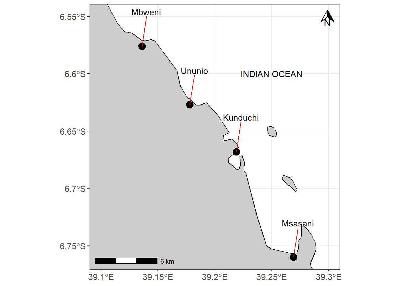
Figure 3.1: Four landing sites in Kinondoni Districts that were selected for this study
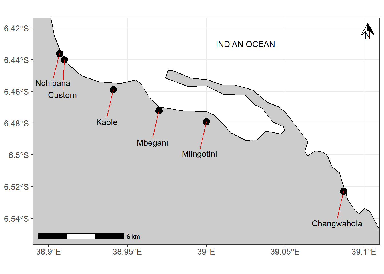
Figure 3.2: Six landing sites in Bagamoyo Districts that were selected for this study
3.2 Mapping
One among the requirements for mapping is the coordinate points; the geographical coordinates of ten fish landing sites in the study area were collected. A field visit was done and longitude and latitude as geographical points for each landing site was recorded using hand held Geographical Positioning System (GPS) unit. These points were exported from GPS unit to Drawing Exchange Format (DXF) using Garmin MapSource software to and later converted to GIS compatible vector format (shapefile) in SAGA, GIS software. The setups of Garmin MapSource were first synchronized with those of GPS unit to WGS84 as a datum using longitude and latitude (in decimal degree) as a geographical position.
The basemap datasets, which included administration boundary, habitat, hydrology, infrastructure and settlement of the study area, were obtained from Institute of Marine Sciences (IMS) GIS database and DIVA-GIS website (http://www.diva-gis.org/gdata). All spatial datasets were converted to feature class and stored in a person geodatabase; an ArcGIS platform for storing feature datasets and a way of organizing related feature class. The road network from IMS database was upgraded using Google Earth images of 2010. Google earth image were georeferenced (Aligned to a known coordinate system) first and later combined in ArcMap using Mosaic tool forming a composite image. New roads were created by importing the composite image in ArcMap and traced over the feature of interest (digitize) using Edit Tool.
3.3 Determine the length of the Coastline
A coastline dataset available from the World Vector Shoreline (WVS) was much generalized, summarized complex Tanzania’s coastline into a simple line for display, and hence was not suitable for measuring the length of coastline for small scale areas. A detailed coastline for the study area was extracted using high detailed feature class dataset from IMS GIS database. Determination of the length of the coastline was based on the following criteria: 1) the coastline is made up of individual line, which has two or more vertices. 2) The sum of the lengths of the pairs of vertices is aggregated for each individual line, and 3) the sum of the lengths of individual lines was aggregated for coastline. Using ArcMAP, two processes were deployed; first, establishing a line representing a coastline. This was done by converting the polygon feature class of the Bagamoyo and Kinondoni Districts to polyline using “feature to polyline tool” in Data Management toolbox. The polyline feature class was further edited to a single line representing the coastline of the study area. This length of the coastline for the study area was further divided into individual fish landing site using “Split Tool” by taking an equidistant (the same distance apart at every point of the fish landing site) along the coastline.
The second step was to measure the length of the coastline, which was done by using “measuring tool” in ArcMap. The Measurement units of the of the tool was reset from the default map units to kilometers and determined the length by simply clicking directly on the coastline layer of each fish landing site in ArcMap, the results were displayed inside the window of the tool, which made easy to copy and paste them into the attribute table of the coastline feature class. Those portions of the coastline with little possibility for fish vessels to anchor was not considered in determination of the length of the coastline, hence the length presented here is a rough estimate focusing on the fish landing sites and should be used with caution
The Pythagorean Theorem4 was later used to compute the distance between the adjacent fish landing sites along the coastline. Given the two longitude points \((x1, x2)\) and latitude points \((y1, y2)\), the distance \(d\) between these points is given in equation (3.1):
\[ \begin{equation} d = \sqrt{(x_2 - x_1)^2 + (y_2 -y_2)^2} \tag{3.1} \end{equation} \]
3.4 Characteristics of landing sites
Attribute and spatial information which formed the basis for the characteristics were extracted from Fisheries Frame Surveys Database. Fish landing sites were characterized based on the fish related infrastructural facilities found at the site.. Data collected include, number of fishermen, total catch of fish landed, species composition, type and number of fishing gear and fishing vessels, fish catch, fisheries officers, Beach Management Unit, processing and storage facilities; electricity and tap water availability; accessibility; and other fish related activities such as restaurants, boat builders and gear repair, and. For determination of the investment value of landing sites, semi-structured interviews were deployed in each landing sites to obtain the value of different type of fishing vessels and gears. Questionnaires were prepared in English but administered in Swahili. The interview was directed to different stakeholders at the fish landing sites including influential fishers, beach recorders, fisheries officers, boat builders and the owners of fishing facilities. Collected data was processed and converted GIS compatible environment and then populated in feature class datasets stored in a personal geodatabase.
3.5 Density of fishing Vessels
According to ESRI, 2008, density in spatial measurements is defined as the quantity per unit area or length. Density of vessel was obtained by taking the total number of fishing vessels divided by the length of the coastline of a particular landing site. The coastline was restricted to study area and fishing vessels were distributed evenly across the length of the coastline.
3.6 Valuing fish landing sites
There are many factors that contribute for wealth of fish landing site, particularly the infrastructural facilities and fish related attributes found at the landing site. It was observed that artisanal fisheries were mostly influenced by fishing vessels, hence, vessels plays and important economical role at the landing site. Essentially two steps were involved for estimating the current vessel’s price and wealth of landing site. Vessel price were obtained by taking the cost of making or buying it. If the price could not be obtained, the price of materials used to make vessels was determined and multiplied with the quantity of the material. The wealth of landing was estimated as the value of fishing vessels multiplied by the number of that particular type of boat for each landing sites. Then the value of each vessel type was summed up to obtain the total investment value of the landing site. Because of the limited availability of data for other attributes, only fishing vessels were considered for estimation of the investment value of the landing site
3.7 Spatial Statistical Analysis
All spatial analyses were performed using Spatial Statistical tools in ArcMap. The spatial analyses assessed the spatial distribution of fish landing sites and determined their spatial pattern. “Average Nearest Neighbor statistical tool was” used for understand the nature of spatial distribution, whether the fish landing sites are clustered in one location, random or dispersed in the study area and also for testing if the distribution pattern is statistical significant.
Spatial pattern of fishing vessels was assessed using Spatial Autocorrection Statistical Tool (Moran’s I), which test the statistical significance of dispersion or clustering of fishing vessels across the study area. Since Moran’s tool give the pattern of distribution but does not show where exactly clustering occur, a Hot Spot Analysis Tool (Getis Ord GI Statistic) was used to investigate which Fish landing sites have high clustering of fishing vessels compared to others. Similarity between and among landing site was determined using a method described by Clarke and Warwick (1994).
References
Richmond, Matthew D. 1997. A Guide to the Seashores of Eastern Africa and the Western Indian Ocean Islands. Sida/Department for Research Cooperation, SAREC.
Semesi, A, Christopher A Muhando, Shigalla B Mahongo, J Daffa, Magnus Ngoile, Yunus D Mgaya, and Julius Francis. 2001. “Coastal Resources and Their Use. In: Eastern Africa Atlas of Coastal Resources.”
A mathematicc rlation in Euclidean geometry that states that the square of the hypotenuse (the side opposite the right angle) is equal to the sum of the squares of the other two sides↩