11 Handling Rasters
When it comes to working with rasters in R, the terra package offers a powerful set of tools. Similar to the sf package, terra provides functions to read and manipulate spatial data. In this case, the focus is on raster data. In this chapter, we will explore the process of handling rasters using the terra package, with a particular emphasis on reading raster files.
11.1 Reading in data
To begin, let’s discuss the central function of the terra package for reading raster files - rast(). This function is designed to handle a wide range of raster file formats, making it a versatile tool for working with raster data. When a raster file is read using rast(), the resulting object is assigned its own class called SpatRaster.
Now, let’s dive into a practical example. Suppose we want to read in a digital elevation model (DEM) for the Western Indian Ocean Region. With the terra package, this process becomes straightforward. We can start by calling the rast() function and providing the path to our raster file as an argument.
First, make sure the terra package is installed and loaded in your R environment:
Once the raster file is read, it is stored in the dem object as a SpatRaster.
class       : SpatRaster
dimensions  : 720, 570, 1  (nrow, ncol, nlyr)
resolution  : 0.01666667, 0.01666667  (x, y)
extent      : 38.49167, 47.99167, -12.00833, -0.008325335  (xmin, xmax, ymin, ymax)
coord. ref. : lon/lat WGS 84 (EPSG:4326)
source      : bathy_ele.tif
name        : wioregio-7753
min value   :         -5040
max value   :          2264
This object contains both the spatial extent of the raster and its associated values. The coord. ref. field shows lon/lat WGS 84, which is Geographic Coordinates. The extent appears to be in degree, with the latitude being a mix of positive and negative numbers. If you just want to know the CRS from a SpatRaster, you just call crs() like so:
[1] "GEOGCRS[\"WGS 84\",\n ENSEMBLE[\"World Geodetic System 1984 ensemble\",\n MEMBER[\"World Geodetic System 1984 (Transit)\"],\n MEMBER[\"World Geodetic System 1984 (G730)\"],\n MEMBER[\"World Geodetic System 1984 (G873)\"],\n MEMBER[\"World Geodetic System 1984 (G1150)\"],\n MEMBER[\"World Geodetic System 1984 (G1674)\"],\n MEMBER[\"World Geodetic System 1984 (G1762)\"],\n MEMBER[\"World Geodetic System 1984 (G2139)\"],\n ELLIPSOID[\"WGS 84\",6378137,298.257223563,\n LENGTHUNIT[\"metre\",1]],\n ENSEMBLEACCURACY[2.0]],\n PRIMEM[\"Greenwich\",0,\n ANGLEUNIT[\"degree\",0.0174532925199433]],\n CS[ellipsoidal,2],\n AXIS[\"geodetic latitude (Lat)\",north,\n ORDER[1],\n ANGLEUNIT[\"degree\",0.0174532925199433]],\n AXIS[\"geodetic longitude (Lon)\",east,\n ORDER[2],\n ANGLEUNIT[\"degree\",0.0174532925199433]],\n USAGE[\n SCOPE[\"Horizontal component of 3D system.\"],\n AREA[\"World.\"],\n BBOX[-90,-180,90,180]],\n ID[\"EPSG\",4326]]"Although the information is a bit disorganized, it does mention the presence of key details such as the datum and and the used World Geodetic System 1984. For instance, we can visualize the DEM using the plot() function from the terra package:
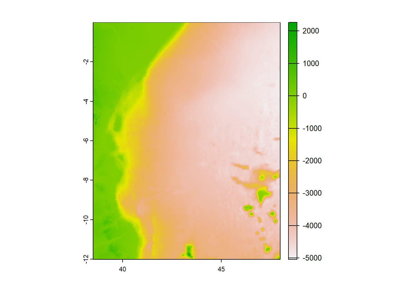
11.2 Glimpse of a raster
With a cell size of 0.01666667 degrees, the equivalent grid size is approximately 1.83km. This information is crucial as it provides insight into the spatial resolution of the raster, which is estimated to be around 1.8km.
SpatExtent : 38.491669165, 47.991671065, -12.008327735, -0.0083253350000021 (xmin, xmax, ymin, ymax)Similarly, observing the geographical extent of the dem file, we can determine that it ranges from approximately 38.49 degrees East to 47.99 degrees East in longitude, and from 12 degrees South to around 0 degrees North in latitude.
[1] 720[1] 570[1] 410400In summary, this raster file contains digital elevation and bathymetry data of the East Africa area. It has a spatial resolution of approximately 1.8km, covering a geographical extent from approximately 38.49 degrees East to 47.99 degrees East in longitude and from 12 degrees South to around 0 degrees North in latitude. The file consists of 720 rows and 570 columns, resulting in a total of 410,400 pixels.
11.3 Cropping
Cropping a raster file to the area of interest is essential for several reasons. Firstly, it helps to reduce the size of the dataset, making it more manageable and efficient to work with, particularly when dealing with large raster files. By focusing only on the area of interest, we can eliminate unnecessary data, thereby improving processing speed and reducing memory usage.
Additionally, cropping allows us to extract specific regions or features that are relevant to our analysis, enabling a more targeted and precise examination of the data. This can enhance the accuracy and reliability of subsequent analyses, as well as facilitate clearer visualization of the specific area under investigation. Ultimately, cropping a raster file to the area of interest streamlines the workflow, optimizes computational resources, and facilitates a more detailed analysis of the desired geographic region.
To crop a raster using the terra package in R, we need first to define the extent for cropping, which determine the extent of the area you want to crop. terra package has a ext function that define the cropping extent by specifying the minimum and maximum values for the x and y coordinates.
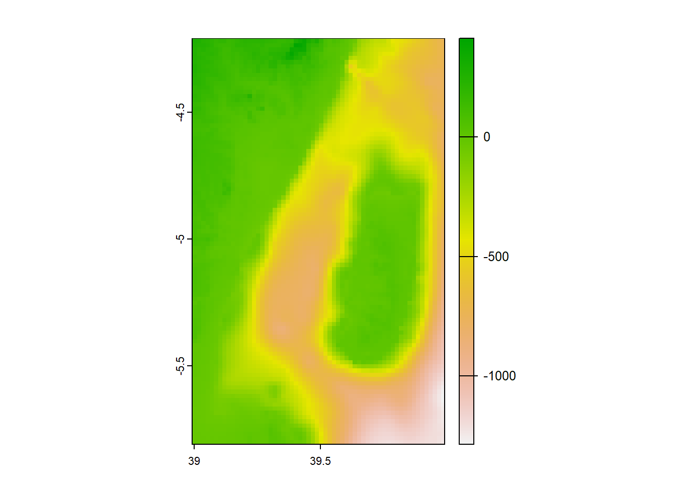
For example, we want to crop the data for the Pemba Channel and hence we can define the geographical cropping extent of the area as;
SpatExtent : 39, 40, -5.8, -4.2 (xmin, xmax, ymin, ymax)Keep your eye on the the ext() function, as it need to follow the order xmin, xmax, ymin, ymax as opposed to xmin, ymin, xmax, ymax as you do for st_crop().
Then we can crop the file using crop() function.
class       : SpatRaster
dimensions  : 96, 60, 1  (nrow, ncol, nlyr)
resolution  : 0.01666667, 0.01666667  (x, y)
extent      : 38.99167, 39.99167, -5.808326, -4.208326  (xmin, xmax, ymin, ymax)
coord. ref. : lon/lat WGS 84 (EPSG:4326)
source(s)   : memory
name        : wioregio-7753
min value   :         -1286
max value   :           413
Notice that the cropped raster for the Pemba Channel has a spatial resolution of approximately 1.8km, which is similar to the origin file but covering a geographical extent from approximately 38.99 degrees East to 39.99 degrees East in longitude and from 5.8 degrees South to around 4.2 degrees South in latitude. The file consists of 96 rows and 60 columns, resulting in a total of 5,760 pixels. The values of raster ranges from 413 to around -1286 meters.
11.4 Classifying rasters
In the terra package, the classify() function allows to assign divide continuous values into discrete or categories of different groups of raster cells based on specified criteria.
To perform raster classification using terra, you typically need a raster object and a classification scheme. The classification scheme defines the rules or conditions to determine how the values in the raster will be categorized. This can be achieved by providing a custom function or a set of thresholds.
We will divide our ocean bathymetry into two groups, all cells with less than or equal to 200 meters are shallow and those cells above 200 as deep
class       : SpatRaster
dimensions  : 96, 60, 1  (nrow, ncol, nlyr)
resolution  : 0.01666667, 0.01666667  (x, y)
extent      : 38.99167, 39.99167, -5.808326, -4.208326  (xmin, xmax, ymin, ymax)
coord. ref. : lon/lat WGS 84 (EPSG:4326)
source(s)   : memory
categories  : wioregio-7753
name        : wioregio-7753
min value   :  (-1300–-200]
max value : (-200–0] 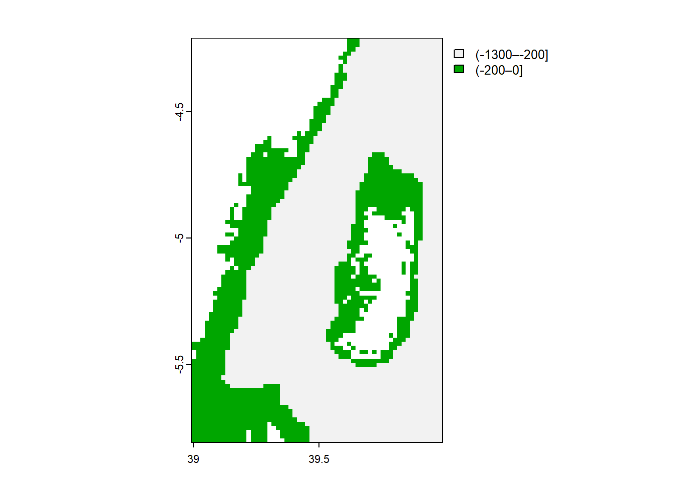
11.5 Aggregating
Adjusting the grid size of raster data, whether by increasing or decreasing it, serves several purposes. Increasing the grid size, or decreasing the resolution, is useful when fine details are not crucial or when working with large datasets, as it reduces computational burden and memory usage. On the other hand, decreasing the grid size, or increasing the resolution, allows for a more precise representation of spatial phenomena, which is advantageous for accurate analyses such as environmental modeling.
Grid size adjustments also aid in data compatibility, harmonizing multiple datasets with different resolutions, and can enhance visualization by simplifying large-scale patterns. Additionally, modifying the grid size can optimize processing efficiency, trading off between detail and computational performance.
The aggregate() function reduces the resolution of the raster by aggregating cells into larger groups. In this case, the fact parameter is set to 5, indicating that each new cell in the aggregated raster will represent a 5x5 grid of the original cells. The fun parameter is set to “mean”, meaning that the values of the cells within each group will be averaged to produce the value of the aggregated cell. This obviously results in some data loss, but that can be acceptable, depending on the purpose of your analysis. Note that you can pass just about any function to fun =, like min(), max() or even your own function.
class       : SpatRaster
dimensions  : 20, 12, 1  (nrow, ncol, nlyr)
resolution  : 0.08333335, 0.08333335  (x, y)
extent      : 38.99167, 39.99167, -5.874993, -4.208326  (xmin, xmax, ymin, ymax)
coord. ref. : lon/lat WGS 84 (EPSG:4326)
source(s)   : memory
name        : wioregio-7753
min value   :      -1202.76
max value   :        258.20
The resulting raster, assigned to the object pemba.dem.low, has a lower resolution compared to the original pemba.dem raster, as cells are combined and averaged.
11.6 Resampling
While the aggregate() function in the terra package is used to increase the grid size and decrease the resolution of a raster, the resample() function is used to modify the grid size and change the resolution of the expected output. By specifying the target resolution or grid size, you can increase or decrease the resolution of the output raster.
To understand the concept of resampling, I am going to demonstrate using the MUR SST product, which has a spatial resolution of approximately 1 kilometer (km). It offers high-resolution global coverage, providing detailed information about sea surface temperature patterns at a fine scale.
Let’s read the file into session
class       : SpatRaster
dimensions  : 201, 301, 1  (nrow, ncol, nlyr)
resolution  : 0.01, 0.01  (x, y)
extent      : 37.995, 41.005, -6.005, -3.995  (xmin, xmax, ymin, ymax)
coord. ref. : lon/lat WGS 84
source      : pemba_mur.nc
varname     : analysed_sst (Analysed Sea Surface Temperature)
name        : analysed_sst
unit        :     degree_C
time        : 2023-06-14 09:00:00 UTC
Upon observation, it becomes apparent that the sea surface temperature (SST) dataset has a resolution of 0.01 degree, which translates to approximately 1.1 kilometers. This resolution is notably higher compared to the 1.8-kilometer resolution of the digital elevation model (DEM).
class       : SpatRaster
dimensions  : 201, 301, 1  (nrow, ncol, nlyr)
resolution  : 0.01, 0.01  (x, y)
extent      : 37.995, 41.005, -6.005, -3.995  (xmin, xmax, ymin, ymax)
coord. ref. : lon/lat WGS 84 (EPSG:4326)
source(s)   : memory
name        : wioregio-7753
min value   :    -1284.7975
max value   :      389.0256
The resampled pemba.dem.high now has a resolution of 0.01 degree, which translates to approximately 1.1 kilometers, the same value to that of sea surface temperature. We can confirm the resolutions using a res function.
[1] 9.166669 9.166669[1] 1.833334 1.833334[1] 1.1 1.1[1] 1.1 1.1Similarly, using the resample() function, it is possible to modify the grid size and adjust the resolution of a raster dataset. In this context, we want to decrease the SST data resolution to align it with the DEM.
class       : SpatRaster
dimensions  : 96, 60, 1  (nrow, ncol, nlyr)
resolution  : 0.01666667, 0.01666667  (x, y)
extent      : 38.99167, 39.99167, -5.808326, -4.208326  (xmin, xmax, ymin, ymax)
coord. ref. : lon/lat WGS 84
source(s)   : memory
name        : analysed_sst
min value   :     -7.76800
max value   :     27.97364
time        : 2023-06-14 09:00:00 UTC
This process ensures that both datasets share a consistent grid size, enabling accurate analysis and comparison between the SST and DEM datasets at a matching resolution.
let’s check whether the extents is the same for temperature and dem
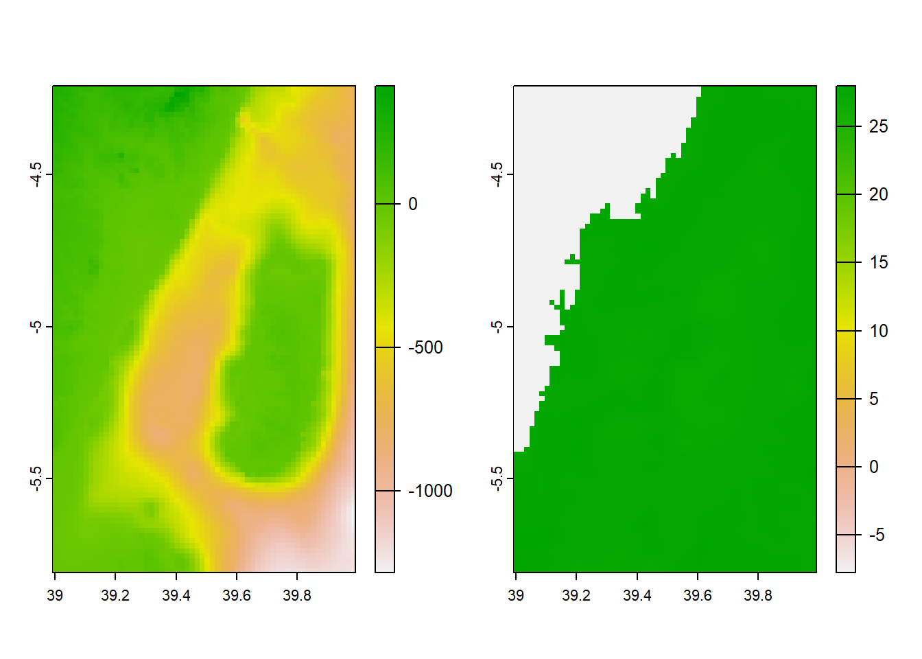
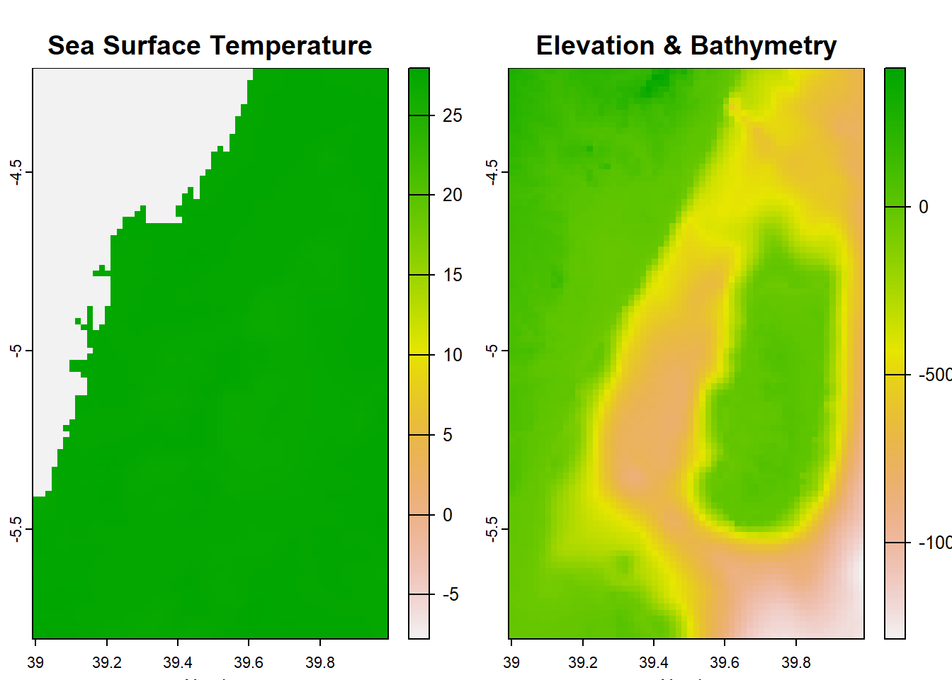
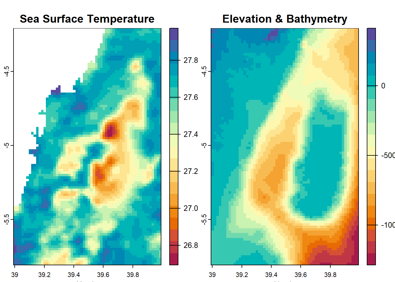
SpatExtent : 38.991669265, 39.991669465, -5.808326495, -4.208326175 (xmin, xmax, ymin, ymax)SpatExtent : 38.991669265, 39.991669465, -5.808326495, -4.208326175 (xmin, xmax, ymin, ymax)We can generate visual representations of the temperature, elevation, and bathymetry variations in the Pemba Channel by plotting the corresponding raster datasets.
11.7 Stacking raster
In terra, you can stack multiple rasters into a single seamless raster object using the c() function, which combines SpatRaster objects as long as they have the same pixel size, extent, and coordinate reference system (CRS) . This is useful when working with multiple rasters that represent different variables or time steps, as it simplifies the reading of raster data by using a single object to represent multiple rasters.
Once we are sure that our raster have similar geographical extents and spatial resolution, we can stack them together using c function in R. This function combines several raster objects into a single stack or brick, enabling simultaneous analysis and manipulation of the stacked layers.
Raster stacking allows for convenient access and processing of multiple layers within a single object, facilitating operations such as extracting values, conducting calculations, or visualizing the combined information. The stacked raster is a useful tool for analyzing and exploring the relationships and variations among different raster datasets in a unified manner.
class       : SpatRaster
dimensions  : 96, 60, 2  (nrow, ncol, nlyr)
resolution  : 0.01666667, 0.01666667  (x, y)
extent      : 38.99167, 39.99167, -5.808326, -4.208326  (xmin, xmax, ymin, ymax)
coord. ref. : lon/lat WGS 84
source(s)   : memory
names       : analysed_sst, wioregio-7753
min values  :     -7.76800,         -1286
max values  :     27.97364,           413
11.8 Basic Plotting
With the dataset size reduced dataset and stacked the file, we can now explore the visualization capabilities offered by the base plotting function. This function, built into R, provides a wide range of options for creating plots and graphs from raster dataset.
11.9 Raster Manipulation
The packages “terra” allow for easy manipulation of raster data in R. With these packages, rasters can be treated as variables in mathematical equations, allowing for exploration of data loss by calculating the difference between original and disaggregated DEMS.
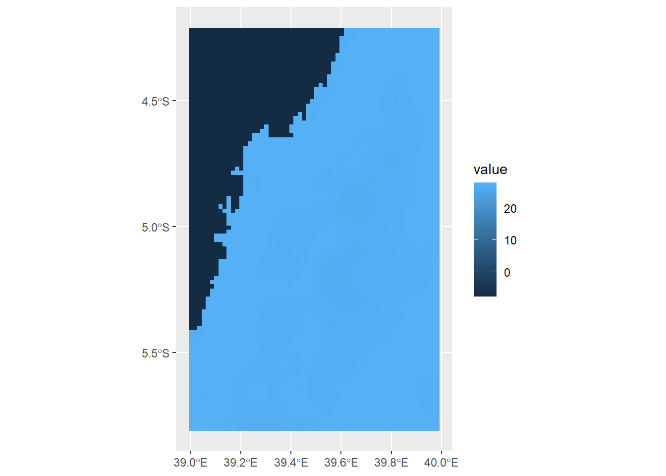
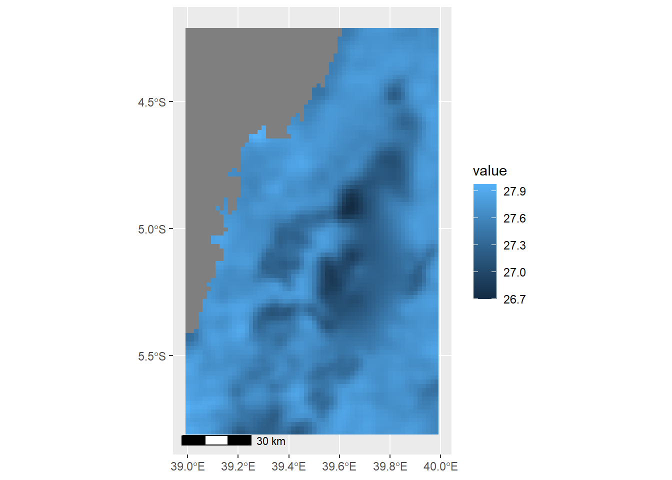
Here we stumble! Why? because this area is close to the equator and hardly find sea surface temperature below 25 degree. But Figure 11.1 indicate a range of temperature from -7 to 28 oC. The color ramp clearly show as the data has the land with darkblue and the ocean with light blue colors, instead of the gradient colors. We should not be fooled by the colors but lets dig the numbers. Lets first check the summary of the raster.
analysed_sst
Min. :-7.768
1st Qu.:27.155
Median :27.561
Mean :20.190
3rd Qu.:27.711
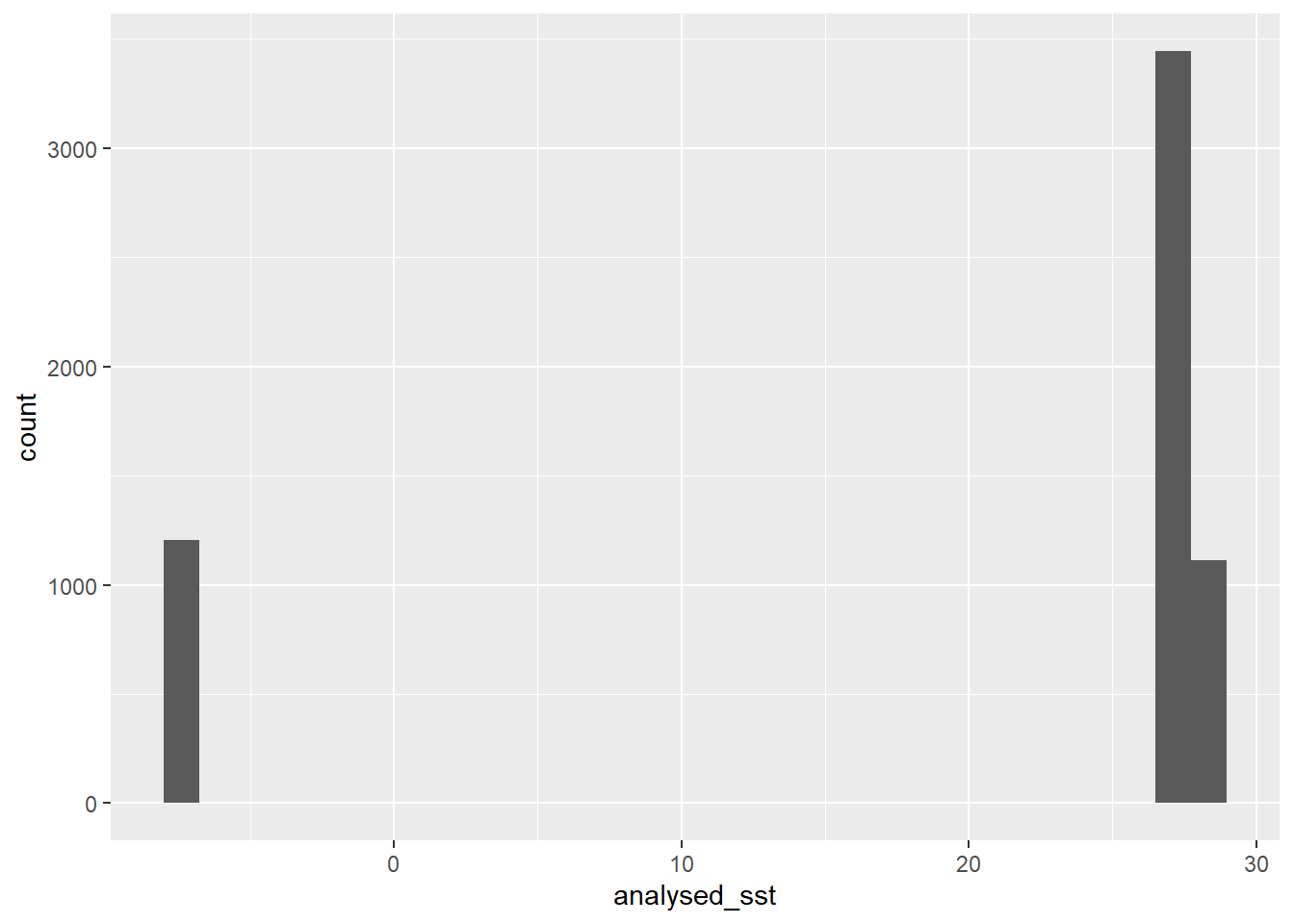
Max. :27.974 We notice that from the first quantile through the maximum value are less than one degree celcius, but the minimum values is far low. Then we spot this as outlier. Let’s us make a histogram of the sst from the raster
class : SpatRaster
dimensions : 96, 60, 1 (nrow, ncol, nlyr)
resolution : 0.01666667, 0.01666667 (x, y)
extent : 38.99167, 39.99167, -5.808326, -4.208326 (xmin, xmax, ymin, ymax)
coord. ref. : lon/lat WGS 84
source(s) : memory
name : sst
min value : 26.69426
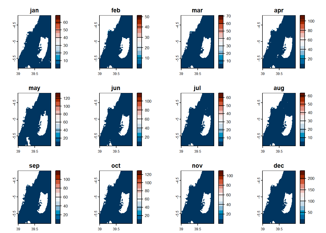
max value : 27.97364 Now the raster file has correct temperature range between 26 and 28 degree celcius. we can make a plot to see the spatial distribution of this temperature in the channel
Code
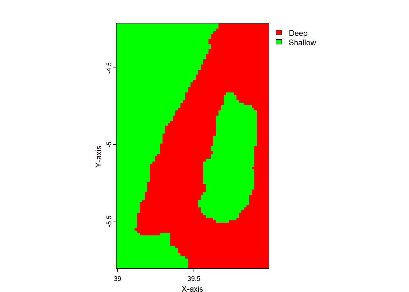
We can use mutate together with if_else function to classify raster based on a threshold value. For instance, we know from literature that artisanal fisheries operated within shallow water of less than 200 meters. Hence, we need to demarcate this area for fisheries management plans. Instead of using mutate, which add raster to existing raster to form stacked raster object, transmute create a raster with only computed values.
Code
class       : SpatRaster
dimensions  : 96, 60, 1  (nrow, ncol, nlyr)
resolution  : 0.01666667, 0.01666667  (x, y)
extent      : 38.99167, 39.99167, -5.808326, -4.208326  (xmin, xmax, ymin, ymax)
coord. ref. : lon/lat WGS 84
source(s)   : memory
categories  : label
name        : bath.class
min value   :       Deep
max value   :    Shallow
Code
To visualize data in R, you can use the ggplot2 package, which provides a flexible and powerful system for creating graphics[1][2]. The ggplot2 package uses a grammar of graphics that allows you to build complex plots by combining simple components[1]. However, if you prefer to use the base plotting function in R, you can do so by using the plot() function in terra[3]. The plot() function creates a map of the values of a SpatRaster or SpatVector object, which can be customized using the available arguments[3]. Overall, both ggplot2 and plot() are useful tools for visualizing data in R, and the choice of which one to use depends on personal preference and the specific needs of the analysis.
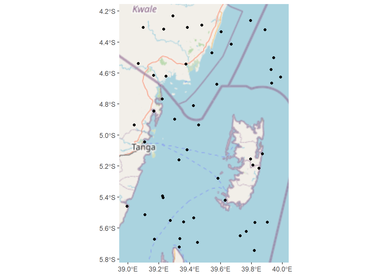
11.10 Point Extraction
Code
chl = list.files("data/satellite data/Chl-a/", pattern = ".nc", full.names = TRUE)
sst = list.files("data/satellite data/SST/", pattern = ".nc", full.names = TRUE)


for (i in 1:12){

label = paste0("data/satellite data/processed/","chl_",month.abb[i] %>% str_to_lower(), ".tif")
label2 = paste0("data/satellite data/processed/","sst_",month.abb[i] %>% str_to_lower(), ".tif")

chl[i] %>%
  terra::rast() %>%
  tidyterra::select(chl = 2) %>%
  # tidyterra::filter(chl < 10) %>%
  # terra::crop(pemba.dem)  %>%
  terra::writeRaster(filename = label)

labe2 = paste0("data/satellite data/processed/","sst_",month.abb[i] %>% str_to_lower(), ".tif")

sst[i] %>%
  terra::rast() %>%
  tidyterra::select(sst = 1) %>%
  # tidyterra::filter(chl < 10) %>%
  # terra::crop(pemba.dem)  %>%
  terra::writeRaster(filename = label2)


}
Code
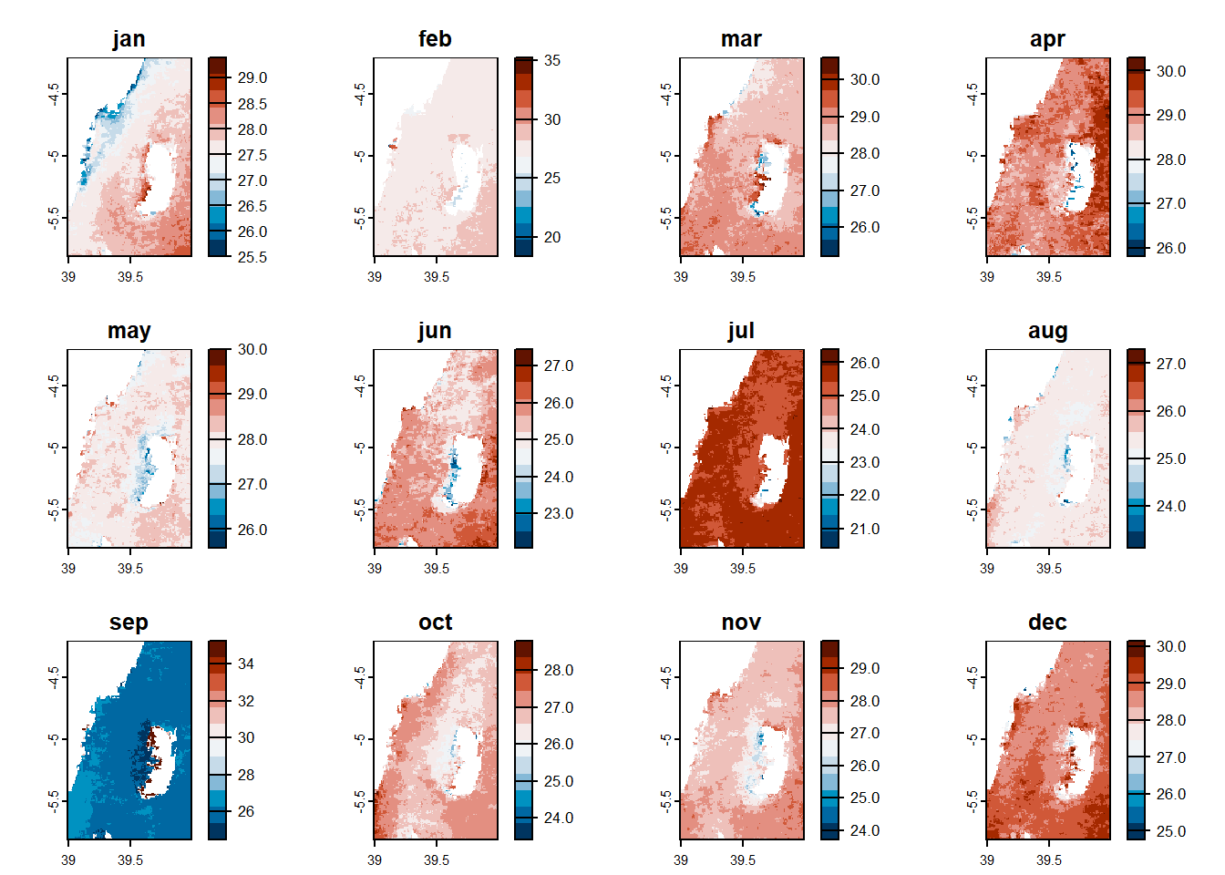
sst.list = list.files(path = "data/satellite data/processed/", pattern = "sst", include.dirs = TRUE, full.names = TRUE)

sst.stack = sst.list %>%
  terra::rast()

sst.stack = sst.stack %>%
  tidyterra::select(
    jan = 5,  feb = 4, mar = 8, apr = 1, may = 9, jun = 7, jul = 6, aug = 2, sep = 12, oct = 11, nov = 10, dec = 3
  )
Code
chl.list = list.files(path = "data/satellite data/processed/", pattern = "chl", include.dirs = TRUE, full.names = TRUE)

chl.stack = chl.list %>%
  terra::rast()

chl.stack = chl.stack %>%
  tidyterra::select(
    jan = 5,  feb = 4, mar = 8, apr = 1, may = 9, jun = 7, jul = 6, aug = 2, sep = 12, oct = 11, nov = 10, dec = 3
  )
Code
Code
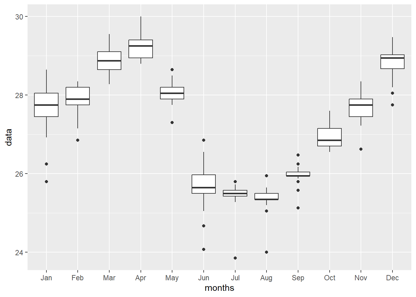
11.10.1 Temperature monthly
Code
random.locations.coords %>%
  bind_cols(
    pemba.sst.locations
  ) %>%
  gt::gt()%>%
  gt::opt_interactive(
    use_search = TRUE,
    # use_filters = TRUE,
    use_resizers = TRUE,
    use_highlight = TRUE,
    use_compact_mode = TRUE,
    use_text_wrapping = FALSE,
    use_page_size_select = TRUE
  ) %>%
  gt::fmt_number(decimals = 3) |>
  gt::fmt_integer(ID) |>
  gt::cols_label_with(
    fn = ~ janitor::make_clean_names(., case = "all_caps")
  ) |>
  gt::data_color(
    columns = jan:mar,
    palette = "Reds"
  ) |>
  gt::data_color(
    columns = may:sep,
    palette = "Blues"
  ) |>
  gt::data_color(
    columns = nov:dec,
    palette = "Reds"
  )|>
  gt::data_color(
    columns = c(apr, oct),
    palette = "Greens"
  )|>
  gt::tab_style(
    style = cell_fill(color = "gray95"),
    locations = cells_body(columns = c(lon, lat))
  ) |>
  gt::tab_style(
    locations = cells_body(columns = ID),
    style = cell_text(weight = "bold")
  )
?(caption)
11.10.2 Chlorophyll monthly
Code
random.locations.coords %>%
  bind_cols(
    pemba.chl.locations
  ) %>%
  gt::gt()%>%
  gt::opt_interactive(
    use_search = TRUE,
    # use_filters = TRUE,
    use_resizers = TRUE,
    use_highlight = TRUE,
    use_compact_mode = TRUE,
    use_text_wrapping = FALSE,
    use_page_size_select = TRUE
  ) %>%
  gt::fmt_number(decimals = 3) |>
  gt::fmt_integer(ID) |>
  gt::cols_label_with(
    fn = ~ janitor::make_clean_names(., case = "all_caps")
  ) |>
  gt::data_color(
    columns = jan:mar,
    palette = "Reds"
  ) |>
  gt::data_color(
    columns = may:sep,
    palette = "Blues"
  ) |>
  gt::data_color(
    columns = nov:dec,
    palette = "Reds"
  )|>
  gt::data_color(
    columns = c(apr, oct),
    palette = "Greens"
  )|>
  gt::tab_style(
    style = cell_fill(color = "gray95"),
    locations = cells_body(columns = c(lon, lat))
  ) |>
  gt::tab_style(
    locations = cells_body(columns = ID),
    style = cell_text(weight = "bold")
  )
?(caption)
Code
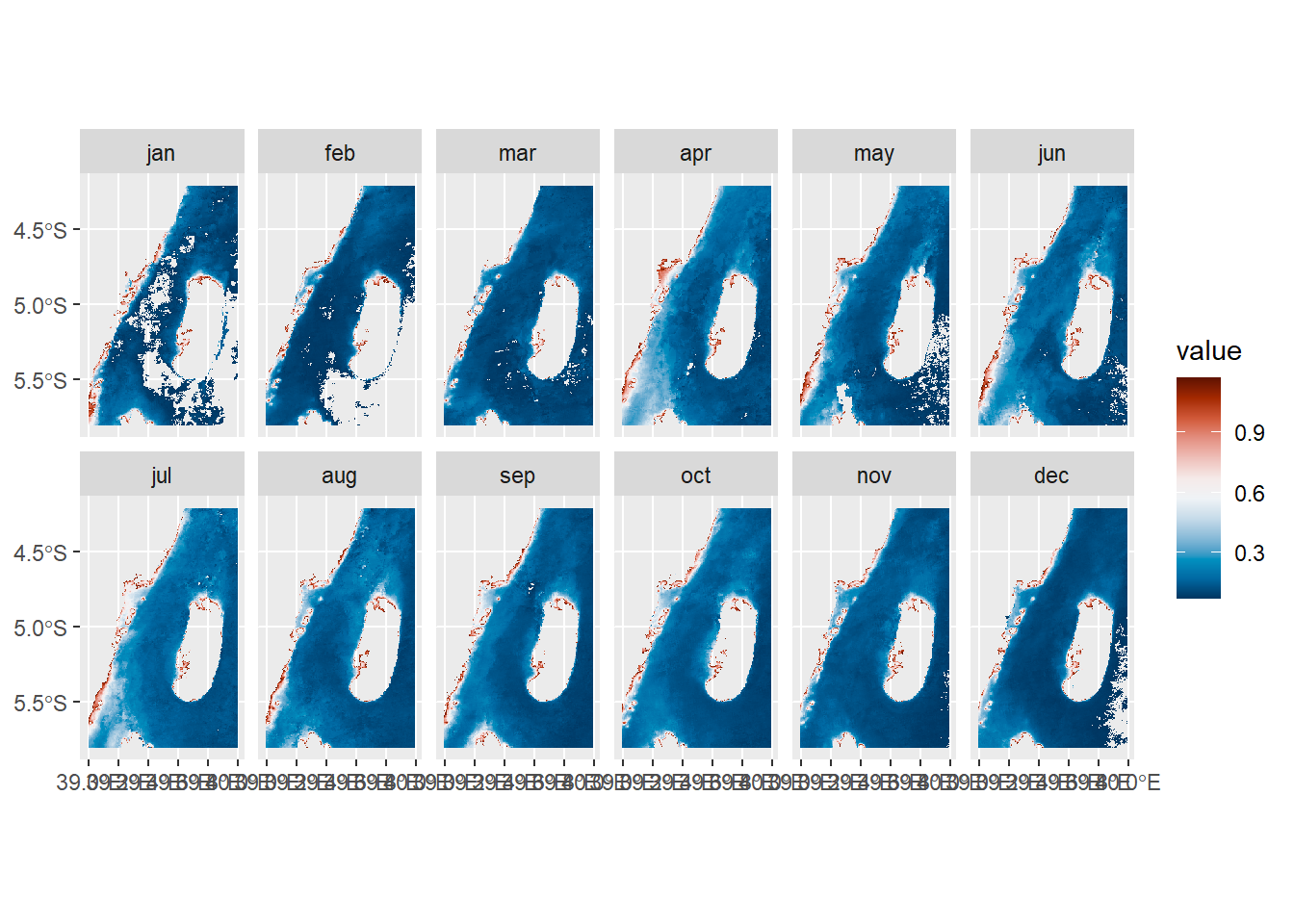
chl.extracts = random.locations.coords %>%
bind_cols(pemba.chl.locations)
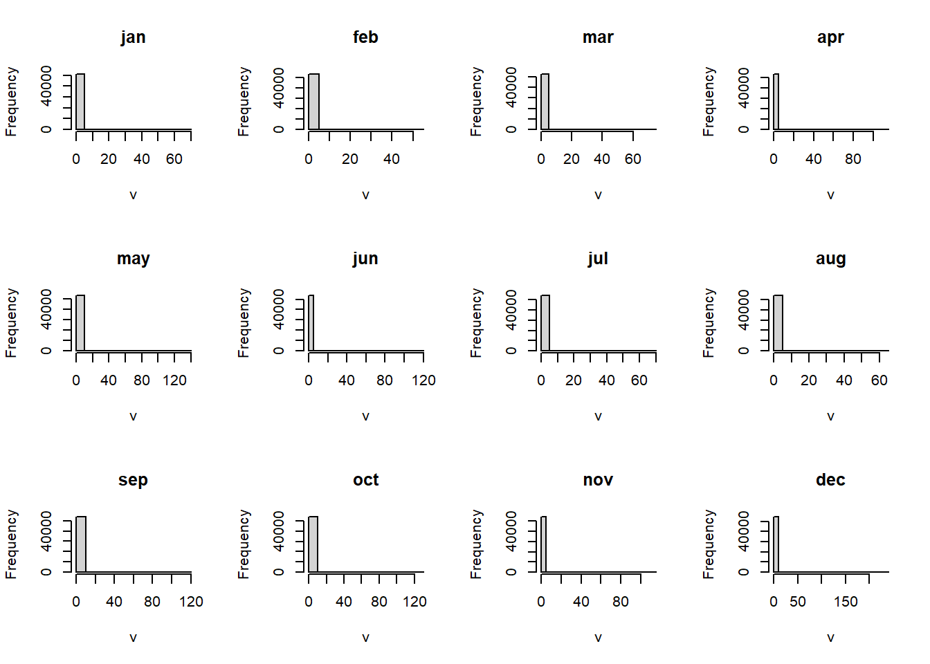
chl.extracts %>%
pivot_longer(cols = jan:dec, names_to = "months", values_to = "data") %>%
mutate(months = str_to_title(months), months = forcats::fct_inorder(months)) %>%
dplyr::filter(data < 1) %>%
ggplot(aes(x = months, y = data))+
geom_boxplot()+
scale_y_continuous(trans = scales::log10_trans())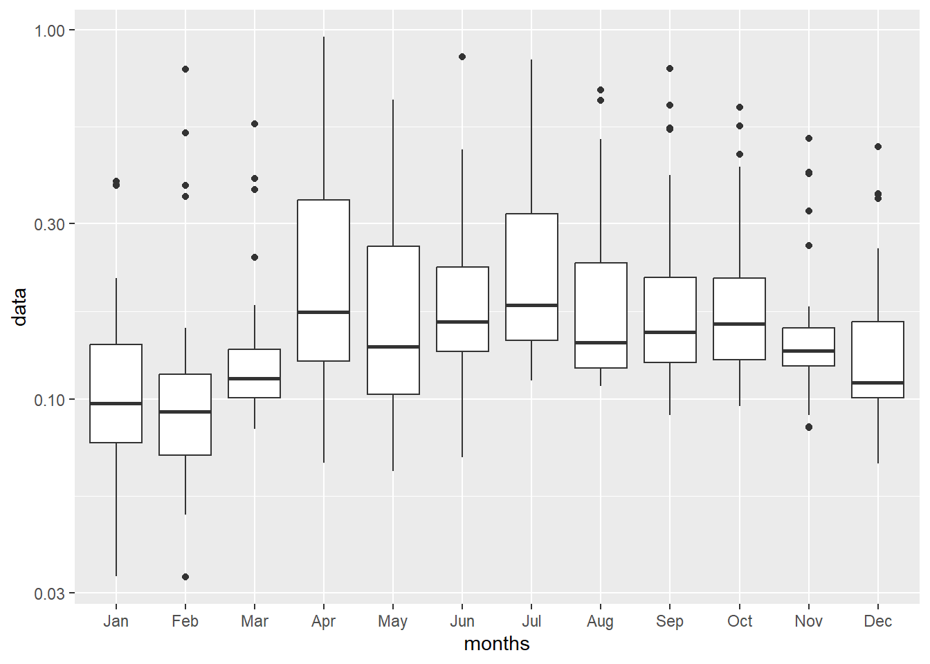
11.11 Raster conversion
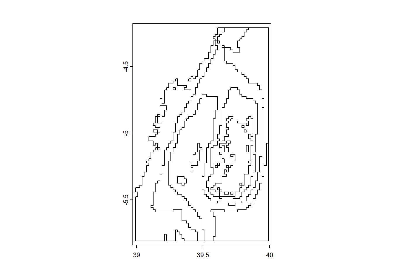
you can derive contour lines as spatVector from bathymetry or elevation raster with as.contour() function
 class       : SpatVector
 geometry    : lines
 dimensions  : 7, 1  (geometries, attributes)
 extent      : 39, 39.98334, -5.799993, -4.21666  (xmin, xmax, ymin, ymax)
 coord. ref. : lon/lat WGS 84 (EPSG:4326)
 names       : level
 type        : <num>
 values      : -1200
               -1000
                -800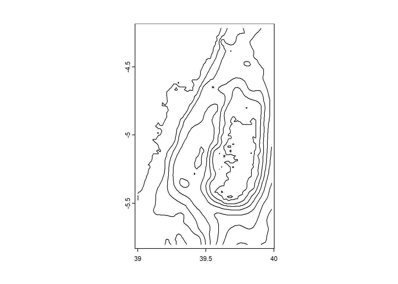
We can also